AI Fairness
There are many different ways of defining what we might look for in a fair machine learning (ML) model. For instance, say we’re working with a model that approves (or denies) credit card applications. Is it:
- fair if the approval rate is equal across genders, or is it
- better if gender is removed from the dataset and hidden from the model?
Four fairness criteria
These four fairness criteria are a useful starting point, but it’s important to note that there are more ways of formalizing fairness, which you are encouraged to explore.
Assume we’re working with a model that selects individuals to receive some outcome. For instance, the model could select people who should be approved for a loan, accepted to a university, or offered a job opportunity. (So, we don’t consider models that perform tasks like facial recognition or text generation, among other things.)
1. Demographic parity / statistical parity
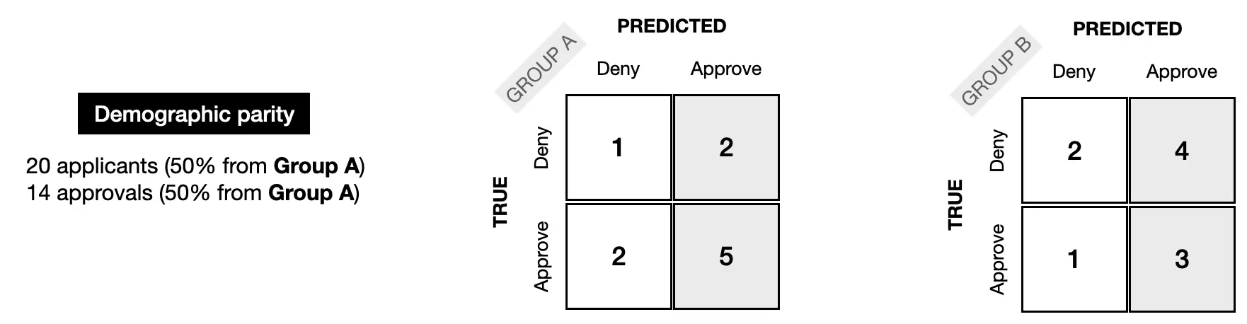
Demographic parity says the model is fair if the composition of people who are selected by the model matches the group membership percentages of the applicants.
A nonprofit is organizing an international conference, and 20,000 people have signed up to attend. The organizers write a ML model to select 100 attendees who could potentially give interesting talks at the conference. Since 50% of the attendees will be women (10,000 out of 20,000), they design the model so that 50% of the selected speaker candidates are women.
2. Equal opportunity
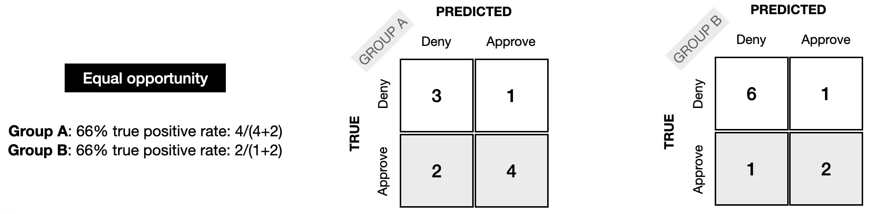
Equal opportunity fairness ensures that the proportion of people who should be selected by the model (“positives”) that are correctly selected by the model is the same for each group. We refer to this proportion as the true positive rate (TPR) or sensitivity of the model.
A doctor uses a tool to identify patients in need of extra care, who could be at risk for developing serious medical conditions. (This tool is used only to supplement the doctor’s practice, as a second opinion.) It is designed to have a high TPR that is equal for each demographic group.
3. Equal accuracy
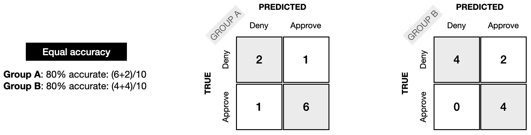
Alternatively, we could check that the model has equal accuracy for each group. That is, the percentage of correct classifications (people who should be denied and are denied, and people who should be approved who are approved) should be the same for each group. If the model is 98% accurate for individuals in one group, it should be 98% accurate for other groups.
A bank uses a model to approve people for a loan. The model is designed to be equally accurate for each demographic group: this way, the bank avoids approving people who should be rejected (which would be financially damaging for both the applicant and the bank) and avoid rejecting people who should be approved (which would be a failed opportunity for the applicant and reduce the bank’s revenue).
4. Group unaware / “Fairness through unawareness”
Group unaware fairness removes all group membership information from the dataset. For instance, we can remove gender data to try to make the model fair to different gender groups. Similarly, we can remove information about race or age.
One difficulty of applying this approach in practice is that one has to be careful to identify and remove proxies for the group membership data. For instance, in cities that are racially segregated, zip code is a strong proxy for race. That is, when the race data is removed, the zip code data should also be removed, or else the ML application may still be able to infer an individual’s race from the data. Additionally, group unaware fairness is unlikely to be a good solution for historical bias.
Example
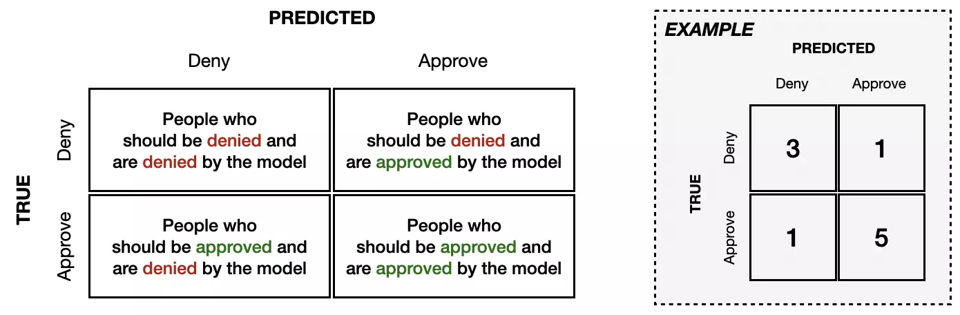
We’ll work with a small example to illustrate the differences between the four different types of fairness. We’ll use a confusion matrix, which is a common tool used to understand the performance of a ML model. This tool is depicted in the example below, which depicts a model with 80% accuracy (since 8/10 people were correctly classified) and has an 83% true positive rate (since 5/6 “positives” were correctly classified).
To understand how a model’s performance varies across groups, we can construct a different confusion matrix for each group. In this small example, we’ll assume that we have data from only 20 people, equally split between two groups (10 from Group A, and 10 from Group B).
The next image shows what the confusion matrices could look like, if the model satisfies demographic parity fairness. 10 people from each group (50% from Group A, and 50% from Group B) were considered by the model. 14 people, also equally split across groups (50% from Group A, and 50% from Group B) were approved by the model.
For equal opportunity fairness, the TPR for each group should be the same; in the example below, it is 66% in each case.
Next, we can see how the confusion matrices might look for equal accuracy fairness. For each group, the model was 80% accurate.
Note that group unaware fairness cannot be detected from the confusion matrix, and is more concerned with removing group membership information from the dataset.
Take the time now to study these toy examples, and use it to build your intuition for the differences between the different types of fairness. How does the example change if Group A has double the number of applicants of Group B?
Also note that none of the examples satisfy more than one type of fairness. For instance, the demographic parity example does not satisfy equal accuracy or equal opportunity. Take the time to verify this now. In practice, it is not possible to optimize a model for more than one type of fairness: to read more about this, explore the Impossibility Theorem of Machine Fairness. So which fairness criterion should you select, if you can only satisfy one? As with most ethical questions, the correct answer is usually not straightforward, and picking a criterion should be a long conversation involving everyone on your team.
When working with a real project, the data will be much, much larger. In this case, confusion matrices are still a useful tool for analyzing model performance. One important thing to note, however, is that real-world models typically cannot be expected to satisfy any fairness definition perfectly. For instance, if “demographic parity” is chosen as the fairness metric, where the goal is for a model to select 50% men, it may be the case that the final model ultimately selects some percentage close to, but not exactly 50% (like 48% or 53%).
Learn more
- Explore different types of fairness with an interactive tool.
- You can read more about equal opportunity in this blog post.
- Analyze ML fairness with this walkthrough of the What-If Tool, created by the People and AI Research (PAIR) team at Google. This tool allows you to quickly amend an ML model, once you’ve picked the fairness criterion that is best for your use case.
We work with a synthetic dataset of information submitted by credit card applicants.
import pandas as pd
from sklearn.model_selection import train_test_split

# Load the data, separate features from target
data = pd.read_csv("../input/synthetic-credit-card-approval/synthetic_credit_card_approval.csv")
X = data.drop(["Target"], axis=1)
y = data["Target"]

# Break into training and test sets
X_train, X_test, y_train, y_test = train_test_split(X, y, train_size=0.8, test_size=0.2, random_state=0)

# Preview the data
print("Data successfully loaded!\n")
X_train.head()
| Num_Children | Group | Income | Own_Car | Own_Housing | |
|---|---|---|---|---|---|
| 288363 | 1 | 1 | 40690 | 0 | 1 |
| 64982 | 2 | 0 | 75469 | 1 | 0 |
| 227641 | 1 | 1 | 70497 | 1 | 1 |
| 137672 | 1 | 1 | 61000 | 0 | 0 |
| 12758 | 1 | 1 | 56666 | 1 | 1 |
The dataset contains, for each applicant:
- income (in the Income column),
- the number of children (in the Num_Children column),
- whether the applicant owns a car (in the Own_Car column, the value is 1 if the applicant owns a car, and is else 0), and
- whether the applicant owns a home (in the Own_Housing column, the value is 1 if the applicant owns a home, and is else 0)
When evaluating fairness, we’ll check how the model performs for users in different groups, as identified by the Group column:
The Group column breaks the users into two groups (where each group corresponds to either 0 or 1). For instance, you can think of the column as breaking the users into two different races, ethnicities, or gender groupings. If the column breaks users into different ethnicities, 0 could correspond to a non-Hispanic user, while 1 corresponds to a Hispanic user.
from sklearn import tree
from sklearn.metrics import confusion_matrix, ConfusionMatrixDisplay
import matplotlib.pyplot as plt

# Train a model and make predictions
model_baseline = tree.DecisionTreeClassifier(random_state=0, max_depth=3)
model_baseline.fit(X_train, y_train)
preds_baseline = model_baseline.predict(X_test)

# Function to plot confusion matrix
def plot_confusion_matrix(estimator, X, y_true, y_pred, display_labels=["Deny", "Approve"],
                          include_values=True, xticks_rotation='horizontal', values_format='',
                          normalize=None, cmap=plt.cm.Blues):
    cm = confusion_matrix(y_true, y_pred, normalize=normalize)
    disp = ConfusionMatrixDisplay(confusion_matrix=cm, display_labels=display_labels)
    return cm, disp.plot(include_values=include_values, cmap=cmap, xticks_rotation=xticks_rotation,
                     values_format=values_format)

# Function to evaluate the fairness of the model
def get_stats(X, y, model, group_one, preds):

    y_zero, preds_zero, X_zero = y[group_one==False], preds[group_one==False], X[group_one==False]
    y_one, preds_one, X_one = y[group_one], preds[group_one], X[group_one]

    print("Total approvals:", preds.sum())
    print("Group A:", preds_zero.sum(), "({}% of approvals)".format(round(preds_zero.sum()/sum(preds)*100, 2)))
    print("Group B:", preds_one.sum(), "({}% of approvals)".format(round(preds_one.sum()/sum(preds)*100, 2)))

    print("\nOverall accuracy: {}%".format(round((preds==y).sum()/len(y)*100, 2)))
    print("Group A: {}%".format(round((preds_zero==y_zero).sum()/len(y_zero)*100, 2)))
    print("Group B: {}%".format(round((preds_one==y_one).sum()/len(y_one)*100, 2)))

    cm_zero, disp_zero = plot_confusion_matrix(model, X_zero, y_zero, preds_zero)
    disp_zero.ax_.set_title("Group A")
    cm_one, disp_one = plot_confusion_matrix(model, X_one, y_one, preds_one)
    disp_one.ax_.set_title("Group B")

    print("\nSensitivity / True positive rate:")
    print("Group A: {}%".format(round(cm_zero[1,1] / cm_zero[1].sum()*100, 2)))
    print("Group B: {}%".format(round(cm_one[1,1] / cm_one[1].sum()*100, 2)))

# Evaluate the model
get_stats(X_test, y_test, model_baseline, X_test["Group"]==1, preds_baseline)
Total approvals: 38246
Group A: 8028 (20.99% of approvals)
Group B: 30218 (79.01% of approvals)

Overall accuracy: 94.79%
Group A: 94.56%
Group B: 95.02%

Sensitivity / True positive rate:
Group A: 77.23%
Group B: 98.03%
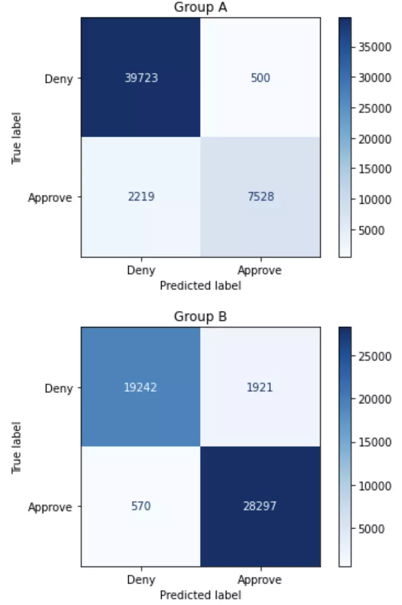
The confusion matrices above show how the model performs on some test data. We also print additional information (calculated from the confusion matrices) to assess fairness of the model. For instance,
- The model approved 38246 people for a credit card. Of these individuals, 8028 belonged to Group A, and 30218 belonged to Group B.
- The model is 94.56% accurate for Group A, and 95.02% accurate for Group B. These percentages can be calculated directly from the confusion matrix; for instance, for Group A, the accuracy is (39723+7528)/(39723+500+2219+7528).
- The true positive rate (TPR) for Group A is 77.23%, and the TPR for Group B is 98.03%. These percentages can be calculated directly from the confusion matrix; for instance, for Group A, the TPR is 7528/(7528+2219).
1) Varieties of fairness
Consider three different types of fairness covered in the tutorial:
- Demographic parity: Which group has an unfair advantage, with more representation in the group of approved applicants? (Roughly 50% of applicants are from Group A, and 50% of applicants are from Group B.)
- Equal accuracy: Which group has an unfair advantage, where applicants are more likely to be correctly classified?
- Equal opportunity: Which group has an unfair advantage, with a higher true positive rate?
All of the fairness criteria are unfairly biased in favor of Group B. 79.01% of applicants are from Group B – if demographic parity is our fairness criterion, fair would mean that 50% of the applicants are from Group B. The model is also slightly more accurate for applicants from Group B (with accuracy of 95.02%, vs 94.56% for Group A). The true positive rate is very high for Group B (98.03%, vs. 77.23% for Group A). In other words, for Group B, almost all people who should be approved are actually approved. For Group A, if you should be approved, your chances of actually being approved are much lower.
def visualize_model(model, feature_names, class_names=["Deny", "Approve"], impurity=False):
    plot_list = tree.plot_tree(model, feature_names=feature_names, class_names=class_names, impurity=impurity)
    [process_plot_item(item) for item in plot_list]

def process_plot_item(item):
    split_string = item.get_text().split("\n")
    if split_string[0].startswith("samples"):
        item.set_text(split_string[-1])
    else:
        item.set_text(split_string[0])

plt.figure(figsize=(20, 6))
plot_list = visualize_model(model_baseline, feature_names=X_train.columns)
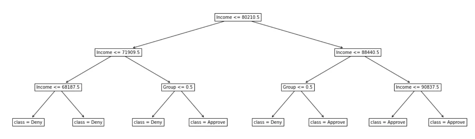
The flowchart shows how the model makes decisions:
- Group <= 0.5 checks what group the applicant belongs to: if the applicant belongs to Group A, then Group <= 0.5 is true.
- Entries like Income <= 80210.5 check the applicant’s income.
To follow the flow chart, we start at the top and trace a path depending on the details of the applicant. If the condition is true at a split, then we move down and to the left branch. If it is false, then we move to the right branch.
For instance, consider an applicant in Group B, who has an income of 75k. Then,
- We start at the top of the flow chart. the applicant has an income of 75k, so Income <= 80210.5 is true, and we move to the left.
- Next, we check the income again. Since Income <= 71909.5 is false, we move to the right.
- The last thing to check is what group the applicant belongs to. The applicant belongs to Group B, so Group <= 0.5 is false, and we move to the right, where the model has decided to approve the applicant.
2) Understand the baseline model
Based on the visualization, how can you explain one source of unfairness in the model?
For all applicants with income between 71909.5 and 88440.5, the model’s decision depends on group membership: the model approves applicants from Group B and denies applicants from Group A. Since we want the model to treat individuals from Group A and Group B fairly, this is clearly a bad model. Although this data is very simple, in practice, with much larger data, visualizing the how a model makes decisions can be very useful to more deeply understand what might be going wrong with a model.
Next, you decide to remove group membership from the training data and train a new model. Do you think this will make the model treat the groups more equally?
# Create new dataset with gender removed
X_train_unaware = X_train.drop(["Group"],axis=1)
X_test_unaware = X_test.drop(["Group"],axis=1)

# Train new model on new dataset
model_unaware = tree.DecisionTreeClassifier(random_state=0, max_depth=3)
model_unaware.fit(X_train_unaware, y_train)

# Evaluate the model
preds_unaware = model_unaware.predict(X_test_unaware)
get_stats(X_test_unaware, y_test, model_unaware, X_test["Group"]==1, preds_unaware)
Total approvals: 36670
Group A: 11624 (31.7% of approvals)
Group B: 25046 (68.3% of approvals)

Overall accuracy: 92.66%
Group A: 93.61%
Group B: 91.72%

Sensitivity / True positive rate:
Group A: 93.24%
Group B: 86.21%
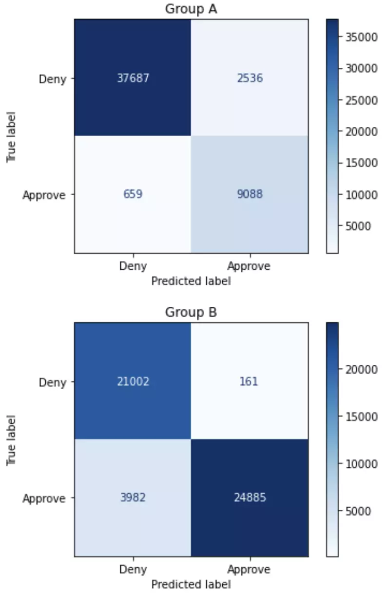
3) Varieties of fairness, part 2
How does this model compare to the first model you trained, when you consider demographic parity, equal accuracy, and equal opportunity? Once you have an answer, run the next code cell.
When we consider demographic parity, the new model is still biased in favor of Group B, but is now a bit more fair than the original model. But now, if you consider either equal accuracy or equal opportunity, the model is biased in favor of Group A! It’s also important to note that the overall accuracy of the model has dropped – for each group, the model is making slightly less accurate decisions.
You decide to train a third potential model, this time with the goal of having each group have even representation in the group of approved applicants. (This is an implementation of group thresholds, which you can optionally read more about here.)
# Change the value of zero_threshold to hit the objective
zero_threshold = 0.11
one_threshold = 0.99

# Evaluate the model
test_probs = model_unaware.predict_proba(X_test_unaware)[:,1]
preds_approval = (((test_probs>zero_threshold)*1)*[X_test["Group"]==0] + ((test_probs>one_threshold)*1)*[X_test["Group"]==1])[0]
get_stats(X_test, y_test, model_unaware, X_test["Group"]==1, preds_approval)
Total approvals: 38241
Group A: 19869 (51.96% of approvals)
Group B: 18372 (48.04% of approvals)

Overall accuracy: 79.38%
Group A: 79.74%
Group B: 79.02%

Sensitivity / True positive rate:
Group A: 100.0%
Group B: 63.64%
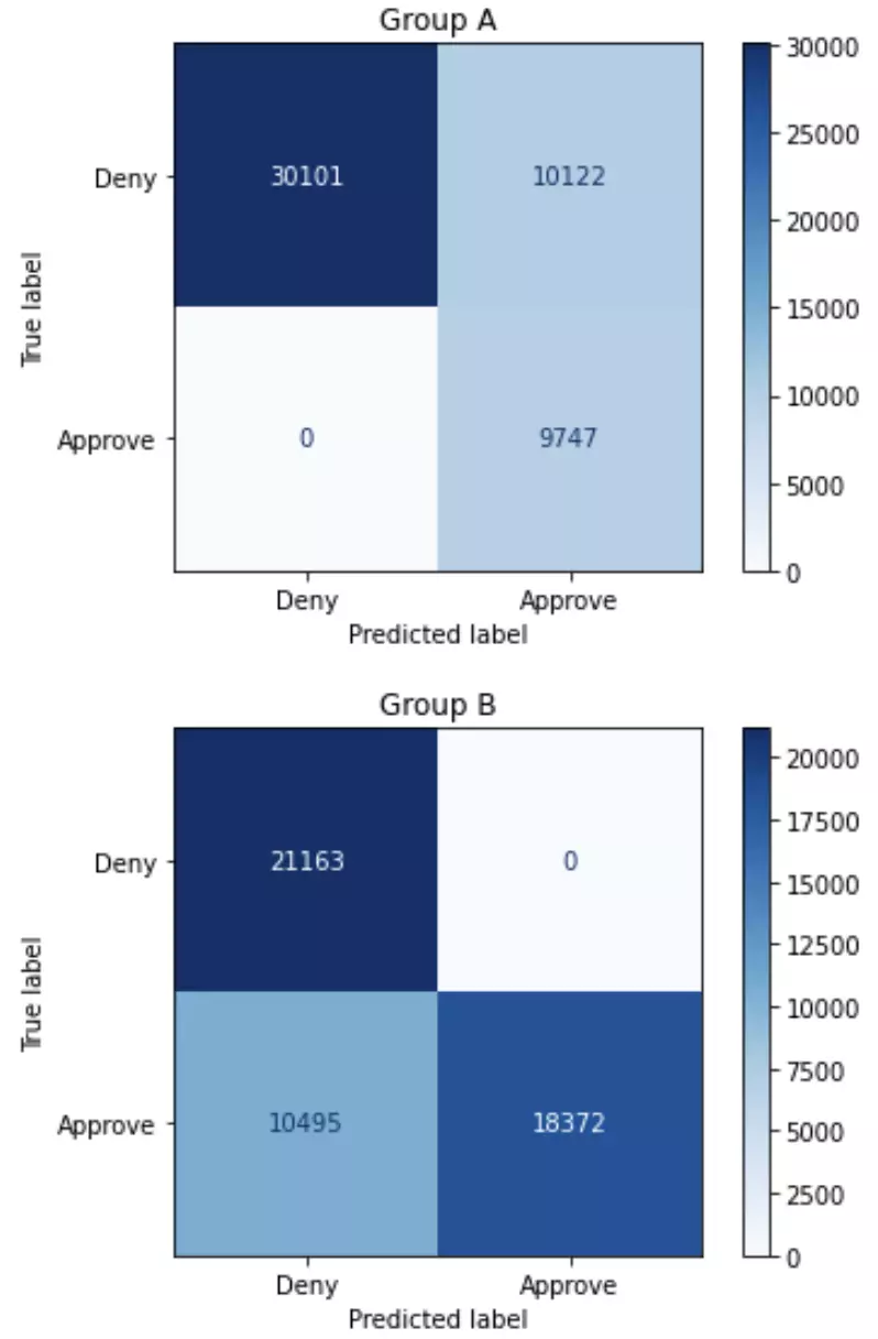
4) Varieties of fairness, part 3
How does this final model compare to the previous models, when you consider demographic parity, equal accuracy, and equal opportunity?
This model acheives nearly equal representation in the pool of approved applicants from each group – if demographic parity is what we care about, then this model is much more fair than the first two models. Accuracy is roughly the same for each group, but there is a substantial drop in overall accuracy for each group. If we examine the model for equal opportunity fairness, the model is biased in favor of Group A: all individuals from Group A who should be approved are approved, whereas only 63% of individuals from Group B who should be approved are approved. (This is similar to the dynamic in the first model, with the favored group switched – that is, in the first model, nearly all individuals from Group B who should be approved were approved by the model.
This is only a short exercise to explore different types of fairness, and to illustrate the tradeoff that can occur when you optimize for one type of fairness over another. We have focused on model training here, but in practice, to really mitigate bias, or to make ML systems fair, we need to take a close look at every step in the process, from data collection to releasing a final product to users.
For instance, if you take a close look at the data, you’ll notice that on average, individuals from Group B tend to have higher income than individuals from Group A, and are also more likely to own a home or a car. Knowing this will prove invaluable to deciding what fairness criterion you should use, and to inform ways to achieve fairness. (For instance, it would likely be a bad aproach, if you did not remove the historical bias in the data and then train the model to get equal accuracy for each group.)