Belief Propogation
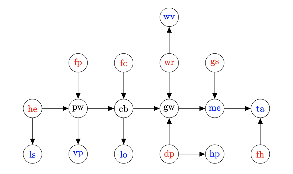
Each row of the data contains a fully observed coffee machine, with the state of every random variable. The random variables are all binary, with \( \texttt{False} \) represented by 0 and \( \texttt{True} \) represented by 1. The variables are:
Failures (we’re trying to detect these):
- he - No electricity
- fp - Fried power supply unit
- fc - Fried circuit board
- wr - Water reservoir empty
- gs - Group head gasket forms seal
- dp - Dead pump
- fh - Fried heating element
Mechanism (these are unobservable):
- pw - Power supply unit works
- cb - Circuit board works
- gw - Get water out of group head
Diagnostic (these are the tests a mechanic can run - observable):
- ls - Room lights switch on
- vp - A voltage is measured across power supply unit
- lo - Power light switches on
- wv - Water visible in reservoir
- hp - Can hear pump
- me - Makes espresso
- ta - Makes a hot, tasty espresso
Above the number is the column number of the provided data (dm, an abbreviation of data matrix) and the two letter code is a suggested variable name.
Coffee Machine Model
If you are unfamiliar with an espresso coffee machine here is a brief description of how one works (you can ignore this):
The user puts ground coffee into a portafilter (round container with a handle and two spouts at the bottom), tamps it (compacts the coffee down), and clamps the portafilter into the group head at the front of the machine. A gasket (rubber ring) forms a seal between the portafilter and group head. A button is pressed. Water is drawn from a reservoir by a pump into a boiler. In the boiler a heating element raises the waters temperature, before the pump pushes it through the group head and into the portafilter at high pressure. The water is forced through the coffee grinds and makes a tasty espresso.
Failures:
- P_he: \( P(\texttt{no electricity}) \)
- P_fp: \( P(\texttt{fried psu}) \)
- P_fc: \( P(\texttt{fried circuit board}) \)
- P_wr: \( P(\texttt{water reservoir empty}) \)
- P_gs: \( P(\texttt{group head gasket seal broken}) \)
- P_dp: \( P(\texttt{dead pump}) \)
- P_fh: \( P(\texttt{fried heating element}) \)
Mechanism:
- P_pw_he_fp: \( P(\texttt{psu works}\mid\texttt{no electricity},\enspace\texttt{fried psu}) \)
- P_cb_pw_fc: \( P(\texttt{circuit board works}\mid\texttt{psu works},\enspace\texttt{fried circuit board}) \)
- P_gw_cb_wr_dp: \( P(\texttt{get water}\mid\texttt{circuit board works},\enspace\texttt{water reservoir empty},\enspace\texttt{dead pump}) \)
Diagnostic:
- P_ls_he: \( P(\texttt{lights switch on}\mid\texttt{no electricity}) \)
- P_vp_pw: \( P(\texttt{voltage across psu}\mid\texttt{psu works}) \)
- P_lo_cb: \( P(\texttt{power light on}\mid\texttt{circuit board works}) \)
- P_wv_wr: \( P(\texttt{water visible}\mid\texttt{water reservoir empty}) \)
- P_hp_dp: \( P(\texttt{can hear pump}\mid\texttt{dead pump}) \)
- P_me_gw_gs: \( P(\texttt{makes espresso}\mid\texttt{get water},\enspace\texttt{group head gasket seal broken}) \)
- P_ta_me_fh: \( P(\texttt{tasty}\mid\texttt{makes espresso},\enspace\texttt{fried heating element}) \)
Note that while the model is close to what you may guess the probabilities are not absolute, to account for mistakes and unknown failures. For instance, the mechanic may make a mistake while brewing an espresso and erroneously conclude that the machine is broken when it is in fact awesome. The probabilities associated with each failure are not uniform. The data set is roughly \( 50:50 \) between failed/working machines, which is hardly realistic for a real product, but makes this exercise simpler as it avoids the problem of extremely rare failure modes.
%matplotlib inline

import zipfile
import io
import csv

from collections import defaultdict
import itertools

import numpy
import matplotlib.pyplot as plt

# Helper used below for some pretty printing, to loop all conditional variable combinations...
# (feel free to ignore)
def loop_conditionals(count):
    if count==0:
        yield (slice(None),)

    else:
        for head in loop_conditionals(count - 1):
            yield head + (0,)
            yield head + (1,)
Loading Data
The below loads the data; it also includes some helpful variables.
# A mapping from the suggested variable names to column indices in the provided file...
nti = dict() # 'name to index'

nti['he'] = 0
nti['fp'] = 1
nti['fc'] = 2
nti['wr'] = 3
nti['gs'] = 4
nti['dp'] = 5
nti['fh'] = 6

nti['pw'] = 7
nti['cb'] = 8
nti['gw'] = 9

nti['ls'] = 10
nti['vp'] = 11
nti['lo'] = 12
nti['wv'] = 13
nti['hp'] = 14
nti['me'] = 15
nti['ta'] = 16

# Opposite to the above - index to name...
itn = ['he', 'fp', 'fc', 'wr', 'gs', 'dp', 'fh',
       'pw', 'cb', 'gw',
       'ls', 'vp', 'lo', 'wv', 'hp', 'me', 'ta'] # 'index to name'

# For conveniance this code loads the data from the zip file,
# so you don't have to decompress it (takes a few seconds to run)...
with zipfile.ZipFile('coffee_machines.zip') as zf:
    with zf.open('coffee_machines.csv') as f:
        sf = io.TextIOWrapper(f)
        reader = csv.reader(sf)
        next(reader)
        dm = []
        for row in reader:
            dm.append([int(v) for v in row])
        dm = numpy.array(dm, dtype=numpy.int8)

# Basic information...
print('Data: {} exemplars, {} features'.format(dm.shape[0], dm.shape[1]))
print('     Broken machines  =', dm.shape[0] - dm[:,nti['ta']].sum())
print('     Working machines =', dm[:,nti['ta']].sum())
Data: 262144 exemplars, 17 features
     Broken machines  = 122603
     Working machines = 139541
Distribution Storage
The below defines storage to represent the probability distributions that are needed to complete the graphical model. A further variable contains a computer readable representation of these variables, for convenience.
# A set of variables that will ultimately represent conditional probability distributions.
# The naming convention is that P_he contains P(he), that P_ta_me_hw contains P(ta|me,hw) etc.
# Indexing is always in the same order that the variables are given in the variables name.

P_he          = numpy.zeros(2)
P_fp          = numpy.zeros(2)
P_fc          = numpy.zeros(2)
P_wr          = numpy.zeros(2)
P_gs          = numpy.zeros(2)
P_dp          = numpy.zeros(2)
P_fh          = numpy.zeros(2)

P_pw_he_fp    = numpy.zeros((2,2,2))
P_cb_pw_fc    = numpy.zeros((2,2,2))
P_gw_cb_wr_dp = numpy.zeros((2,2,2,2))

P_ls_he       = numpy.zeros((2,2))
P_vp_pw       = numpy.zeros((2,2))
P_lo_cb       = numpy.zeros((2,2))
P_wv_wr       = numpy.zeros((2,2))
P_hp_dp       = numpy.zeros((2,2))
P_me_gw_gs    = numpy.zeros((2,2,2))
P_ta_me_fh    = numpy.zeros((2,2,2))

# This list describes the above in a computer readable form,
# as the tuple (numpy array, human readable name, list of RVs, kind);
# the list of RVs is aligned with the dimensions of the numpy array
# and kind is 'F' for failure, 'M' for mechanism and 'D' for diagnostic..
rvs = [(P_he, 'P(he)', [nti['he']], 'F'),
       (P_fp, 'P(fp)', [nti['fp']], 'F'),
       (P_fc, 'P(fc)', [nti['fc']], 'F'),
       (P_wr, 'P(wr)', [nti['wr']], 'F'),
       (P_gs, 'P(gs)', [nti['gs']], 'F'),
       (P_dp, 'P(dp)', [nti['dp']], 'F'),
       (P_fh, 'P(fh)', [nti['fh']], 'F'),
       (P_pw_he_fp, 'P(pw|he,fp)', [nti['pw'], nti['he'], nti['fp']], 'M'),
       (P_cb_pw_fc, 'P(cb|pw,fc)', [nti['cb'], nti['pw'], nti['fc']], 'M'),
       (P_gw_cb_wr_dp, 'P(gw|cb,wr,dp)', [nti['gw'], nti['cb'], nti['wr'], nti['dp']], 'M'),
       (P_ls_he, 'P(ls|he)', [nti['ls'], nti['he']], 'D'),
       (P_vp_pw, 'P(vp|pw)', [nti['vp'], nti['pw']], 'D'),
       (P_lo_cb, 'P(lo|cb)', [nti['lo'], nti['cb']], 'D'),
       (P_wv_wr, 'P(wv|wr)', [nti['wv'], nti['wr']], 'D'),
       (P_hp_dp, 'P(hp|dp)', [nti['hp'], nti['dp']], 'D'),
       (P_me_gw_gs, 'P(me|gw,gs)', [nti['me'], nti['gw'], nti['gs']], 'D'),
       (P_ta_me_fh, 'P(ta|me,fh)', [nti['ta'], nti['me'], nti['fh']], 'D')]
Learning Conditional Probability Distributions
Above, a set of variables representing conditional probability distributions has been defined. They are to represent a Bernoulli trial for each combination of conditional variables, given as \( P(\texttt{False}\mid …) \) in rv[0,...] and \( P(\texttt{True}\mid …) \) in rv[1,...]. Obviously these two values should sum to 1; giving the probability of both \( \texttt{True} \) and \( \texttt{False} \) is redundant, but makes all of the code much cleaner.
The next task is to fill in the distributions with a maximum a posteriori probability (MAP) estimate given the data. The prior to be used for all RVs is a Beta distribution,
\[P(x) \propto x^{\alpha-1}(1-x)^{\beta-1}\]such that \( x \) is the probability of getting a \( \texttt{False} \) from the Bernoulli draw (note that this is backwards from what you might suspect, because it keeps the arrays in the same order). The hyperparameters for the priors are to be set as \( \alpha = \beta = 1 \). The Beta distribution is conjugate, that is when you observe a Bernoulli draw and update using Bayes rule the posterior is also a Beta distribution. This makes the procedure particularly simple:
- Initialise every conditional probability with the hyperparameters \( \alpha \) and \( \beta \)
- Update them for every coffee machine in the data set
- Extract the maximum likelihood parameters from the posterior \( \alpha \) and \( \beta \) parameters
Writing out the relevant parts of the Bayes rule update for observing a RV, \( v = 0 \) (\( \texttt{False} \)), you get
\[\begin{aligned} \operatorname{Beta}(x | \alpha_1, \beta_1) &\propto \operatorname{Bernoulli}(v = 0 | x)\operatorname{Beta}(x | s\alpha_0,\beta_0)\\ x^{\alpha_1-1}(1-x)^{\beta_1-1} &\propto \left(x^{(1-v)} (1-x)^v\right) \left(x^{\alpha_0-1}(1-x)^{\beta_0-1}\right)\\ x^{\alpha_1-1}(1-x)^{\beta_1-1} &\propto x^1 (1-x)^0 x^{\alpha_0-1}(1-x)^{\beta_0-1}\\ x^{\alpha_1-1}(1-x)^{\beta_1-1} &\propto x^{\alpha_0+1-1}(1-x)^{\beta_0-1}\\ \operatorname{Beta}(x | \alpha_1, \beta_1) &= \operatorname{Beta}(x | \alpha_0+1,\beta_0) \end{aligned}\]Subscripts of the hyperparameters are used to indicate how many data points have been seen; True works similarly. Put simply, the result is that you count how many instances exist of each combination, and add 1 for the hyperparameters. The maximum likelihood is then the expected value, which is
\[P(v=\textrm{False}|\ldots) = \frac{\alpha}{\alpha + \beta}\]It’s typical to do all of the above within the conditional probability distribution arrays, using them to represent \( \alpha \) and \( \beta \) then treating step 3 as converting from hyperparameters to expected values.
for i in range(len(rvs)):

    col_index = rvs[i][2]
    probabilities = numpy.argwhere(rvs[i][0] == 0)
    for prob in probabilities:
        prob1 = prob.copy()
        prob1[0] = 1 - prob[0]

        num1 = numpy.all(dm[:,col_index] == prob, axis=1).sum()
        num2 = numpy.all(dm[:,col_index] == prob1, axis=1).sum()

        rvs[i][0][tuple(prob)] = (1 + num1) / (2 + num2 + num1)


# Print out the RVs for a sanity check...
for rv in rvs:
    if len(rv[2])==1:
        print('{} = {}'.format(rv[1], rv[0]))
    else:
        print('{}:'.format(rv[1]))
        for i in loop_conditionals(len(rv[2])-1):
            print('  P({}|{}) = {}'.format(itn[rv[2][0]], ','.join([str(v) for v in i[1:]]), rv[0][i]))
    print()
P(he) = [0.99047096 0.00952904]

P(fp) = [0.80056152 0.19943848]

P(fc) = [0.98004547 0.01995453]

P(wr) = [0.89956742 0.10043258]

P(gs) = [0.95010414 0.04989586]

P(dp) = [0.94968071 0.05031929]

P(fh) = [0.97033714 0.02966286]

P(pw|he,fp):
  P(pw|0,0) = [4.81037502e-06 9.99995190e-01]
  P(pw|0,1) = [9.99980683e-01 1.93173257e-05]
  P(pw|1,0) = [9.99495714e-01 5.04286435e-04]
  P(pw|1,1) = [0.9980695 0.0019305]

P(cb|pw,fc):
  P(cb|0,0) = [9.99981208e-01 1.87916941e-05]
  P(cb|0,1) = [9.99048525e-01 9.51474786e-04]
  P(cb|1,0) = [4.90910787e-06 9.99995091e-01]
  P(cb|1,1) = [9.99760937e-01 2.39062874e-04]

P(gw|cb,wr,dp):
  P(gw|0,0,0) = [9.99980048e-01 1.99517168e-05]
  P(gw|0,0,1) = [9.99611349e-01 3.88651380e-04]
  P(gw|0,1,0) = [9.99817718e-01 1.82282173e-04]
  P(gw|0,1,1) = [0.99630996 0.00369004]
  P(gw|1,0,0) = [5.75251529e-06 9.99994247e-01]
  P(gw|1,0,1) = [9.99892404e-01 1.07596299e-04]
  P(gw|1,1,0) = [0.90239779 0.09760221]
  P(gw|1,1,1) = [9.99056604e-01 9.43396226e-04]

P(ls|he):
  P(ls|0) = [0.09996957 0.90003043]
  P(ls|1) = [9.99599840e-01 4.00160064e-04]

P(vp|pw):
  P(vp|0) = [9.99981572e-01 1.84284240e-05]
  P(vp|1) = [0.01009698 0.98990302]

P(lo|cb):
  P(lo|0) = [9.99982890e-01 1.71101035e-05]
  P(lo|1) = [0.00103582 0.99896418]

P(wv|wr):
  P(wv|0) = [0.19985667 0.80014333]
  P(wv|1) = [9.99962019e-01 3.79809336e-05]

P(hp|dp):
  P(hp|0) = [0.09929465 0.90070535]
  P(hp|1) = [9.99924196e-01 7.58035173e-05]

P(me|gw,gs):
  P(me|0,0) = [9.99987818e-01 1.21821969e-05]
  P(me|0,1) = [9.99768626e-01 2.31374364e-04]
  P(me|1,0) = [0.09908254 0.90091746]
  P(me|1,1) = [0.89921242 0.10078758]

P(ta|me,fh):
  P(ta|0,0) = [9.99990701e-01 9.29903848e-06]
  P(ta|0,1) = [9.99696233e-01 3.03766707e-04]
  P(ta|1,0) = [0.04966799 0.95033201]
  P(ta|1,1) = [9.99777134e-01 2.22866057e-04]
Factor Graph
The graphical model has been given as a Bayesian network, but computation is much simpler on a factor graph (see slides for details, including a visual version of the below algorithm). Inevitably, the first step is to convert; the algorithm to do so is:
- For each RV we need two nodes: The random variable itself and a factor node. There must be an edge connecting them.
- Each conditional distribution generates as many edges as there are conditional terms. Each edge is between the factor associated with the RV and one of the RVs it is conditioned on.
The algorithm itself involves passing messages along the edges, so what we require is a list of edges. Being more specific, the objective is hence to generate that list of edges; an edge is represented by a tuple containing two integers, these being the indices of the nodes that are either side of the edge. For the RVs we can use the indices already provided by nti and used in the rvs list. As factors are paired with RVs the index of the factor node paired with RV \( i \) shall be defined \( i+17 \) (there are 17 RVs, so this puts them immediately after the RVs in the same order).
def rv2fac(i):
    """Given the index of a random variable node this returns the index of
    the corresponding factor node."""
    return i + 17

def fac2rv(i):
    """Given the index of a factor node this returns the index of
    the corresponding random variable node."""
    return i - 17

def calc_edges(rvs):
    """Uses the rvs array to calculate and return a list of edges,
    each as a tuple (index node a, index node b)"""
    edges = []

    for rv in rvs:
        if len(rv[2]) == 1:
            edges.append((rv[2][0], rv2fac(rv[2][0])))
        else:
            node = list(rv)[2][0]
            edges.append((node, rv2fac(node)))
            for connection in list(rv)[2][1:]:
                edges.append((rv2fac(node), connection))

    return edges

edges = calc_edges(rvs)
print('Generated {} edges'.format(len(edges)))
print(edges)
Generated 33 edges
[(0, 17), (1, 18), (2, 19), (3, 20), (4, 21), (5, 22), (6, 23), (7, 24), (24, 0), (24, 1), (8, 25), (25, 7), (25, 2), (9, 26), (26, 8), (26, 3), (26, 5), (10, 27), (27, 0), (11, 28), (28, 7), (12, 29), (29, 8), (13, 30), (30, 3), (14, 31), (31, 5), (15, 32), (32, 9), (32, 4), (16, 33), (33, 15), (33, 6)]
Message Order
Belief propagation works by passing messages over the edges of the factor graph, two messages per edge as there is one in each direction. A message can only be sent from node \( a \) to node \( b \) when node \( a \) has received all of it’s messages, except for the message from node \( b \) to node \( a \), which is not needed for that calculation. For this reason we need to convert the list of edges into a list of messages to send, ordered such that the previous constraint is never violated. Note that this naturally involves doubling the number of items in the list as we now have two entries per edge, one per direction.
There are many ways to solve this problem and you’re welcome to choose any (the below is not the best), but here is a description of an approach that works by simulating message passing where constraints are checked: Generate a list of messages to send (the edges plus the edges with the tuples reversed, to cover both directions) and an empty list, which will ultimately contain the messages in the order they were sent. The algorithm then proceeds by identifying messages in the first list for which the constraint has been satisfied and then moving them to the end of the second list, indicating the message has been sent. This is repeated until the first list is empty and the second full; the second will be in a valid message sending order.
Implemented badly the above is both horrifically slow and fiddly to code. One technique to make it faster is to bounce — instead of going through the list of messages to send in the same order each time you go forwards and then backwards and then forwards etc. This avoids the scenario where the to send list contains the messages in reverse sending order, such that with each loop you only find one more message that you can send, meaning you have to loop as many times as there are messages. A second technique also makes the code much simpler. Figuring out if you can send a message when the lists are represented as lists is slow — you have to loop both. Instead, convert the lists into a pair of nested dictionaries indexed [message destination][message source] (order is important!) that contains \( \texttt{True} \) if the message has been sent (in second list), \( \texttt{False} \) if it has not (in first list). It’s now simple to check if a message can be sent or not; you will still need to generate the list of messages to send as you flip values from \( \texttt{False} \) to \( \texttt{True} \) (make sure you get the order right — the dictionaries are indexed backwards).
def calc_msg_order(edges):
    """Given a list of edges converts to a list of messages such that
    the returned list contains tuples of (source node, destination node)."""

    msgs = []
    current_state = defaultdict(dict)
    for i, j in edges:
        current_state[i][j] = 0
    for i, j in edges:
        current_state[j][i] = 0

    forward = list(current_state)
    backward = list(current_state)[::-1]
    all_messages = forward + backward

    complete = 0
    while not complete:
        complete = 1
        for j in all_messages:
             for i in current_state[j]:
                if current_state[j][i] != 0:
                    continue
                else:
                    if all(v for k, v in current_state[i].items() if k != j):
                        current_state[j][i] = 1
                        msgs.append((i, j))
                    else:
                        complete = 0

    return msgs

msg_order = calc_msg_order(edges)
print('Generated {} messages'.format(len(msg_order)))
print(msg_order)
Generated 66 messages
[(17, 0), (18, 1), (19, 2), (20, 3), (21, 4), (22, 5), (23, 6), (1, 24), (2, 25), (10, 27), (11, 28), (12, 29), (13, 30), (14, 31), (4, 32), (6, 33), (16, 33), (33, 15), (29, 8), (28, 7), (31, 5), (30, 3), (27, 0), (0, 24), (3, 26), (5, 26), (15, 32), (32, 9), (24, 7), (7, 25), (9, 26), (25, 8), (26, 8), (8, 25), (8, 26), (8, 29), (29, 12), (26, 9), (25, 7), (26, 5), (26, 3), (25, 2), (7, 24), (7, 28), (3, 30), (5, 31), (9, 32), (2, 19), (3, 20), (5, 22), (32, 15), (31, 14), (30, 13), (28, 11), (32, 4), (24, 1), (24, 0), (0, 27), (15, 33), (0, 17), (1, 18), (4, 21), (33, 16), (27, 10), (33, 6), (6, 23)]
Message Passing
There are two kinds of node: RVs and factors. The message sent by a random variable is simply all incoming messages multiplied together, except for the message from the direction it is sending a message, i.e.
\[M_{s \rightarrow d}(x) = \prod_{\forall n \cdot n \neq d} M_{n \rightarrow s}(x)\]where \( s \) (source) is a RV and \( d \) (destination) is a factor and \( n \) covers the neighbours of \( s \) (they must each have sent a message to \( s \), and will be factors). \( x \) is 0 or 1, corresponding to \( \texttt{False} \) or \( \texttt{True} \); messages are functions, conveniently discrete and hence represented as arrays in this case. This equation is exactly what you need to evaluate in send_rv(). An almost identical equation is the belief, that is the marginal distribution of a RV and the final output of the algorithm:
\[B_s(x) = \prod_{\forall n} M_{n \rightarrow s}(x)\]In the interest of laziness send_rv should calculate this if the destination is set to None; if implemented in the simplest way this will naturally be the case.
The messages that factors send are more complicated, because they factor in (sorry) the conditional probability distributions:
\[M_{s \rightarrow d}(x_d) = \sum_{\forall x_m \cdot m \neq d} P[s,d,\ldots] \prod_{\forall n \cdot n \neq d} M_{n \rightarrow s}(x_n)\]where \( P[s,d,\ldots] \) is the conditional probability distribution, which will naturally be indexed by the source, destination, and any other neighbours (\( n \)). The switch to \( [\enspace] \) is to indicate that you should stop thinking of it as a probability distribution when passing messages, as some of the messages make no sense when interpreted as such (but the final beliefs always make sense; it’s just the intermediate messages that get weird). The key detail is that this is no longer simple multiplication: Each message is over a different RV (the RV of its source) and hence needs to be multiplied in the correct way. A typical recipe for this is:
- Copy the factor (\(P[s,d,\cdot]\)) so it can be used as working storage
- Multiply in each message to the source (unless from destination), using broadcasting to align it with the correct dimension
- Marginalise out all but the RV of the destination node
def send_rv(src, dest, msgs):
    """Returns the message to send from src (source, always a RV) to dest (destination,
    always a factor). msgs is dictionaries within a dictionary such that [d][s]
    gets you the message from s to d. Because the message sending order is
    correct (well...) you can assume all required entries exist in msgs."""

    # **************************************************************** 1 mark
    send_message_rv = numpy.ones(2)
    for k, v in msgs[src].items():
        if k == dest:
            continue
        else:
            send_message_rv *= v

    return send_message_rv

def send_factor(src, dest, msgs, rvs):
    """Returns the message to send from src (source, always a factor) to dest
    (destination, always a RV). msgs is dictionaries within a dictionary such
    that [d][s] gets you the message from s to d. Because the message sending
    order is correct you can assume all required entries exist in msgs.
    rvs is as defined above and contains the relevant conditional distributions
    and the names of the dimensions"""

    send_message_factor = rvs[fac2rv(src)][0].copy()
    _ = []
    for k, v in msgs[src].items():
        if k == dest:
            continue
        else:
            idx_no = rvs[fac2rv(src)][2].index(k)
            dimensions = []
            for i in range(len(send_message_factor.shape)):
                if i == idx_no:
                    dimensions.append(2)
                else:
                    dimensions.append(1)
            _.append(idx_no)
            send_message_factor *= v.reshape(dimensions)
    send_message_factor = send_message_factor.sum(axis = tuple(_))
    return send_message_factor
Belief Propagation
Once you have the ability to send messages and an order in which to send the messages the rest of the algorithm is a cake walk. The only trick is that if a RV is known (observed) then instead of using send_rv whenever a message is sent from it you send the distribution it is known to be instead (\( [1,0] \) for \( \texttt{False} \), \( [0,1] \) for \( \texttt{True} \)). The below code implements this.
def marginals(known):
    """known is a dictionary, where a random variable index existing as a key in the dictionary
    indicates it has been observed. The value obtained using the key is the value the
    random variable has been observed as. Returns a 17x2 matrix, such that [rv, 0] is the
    probability of random variable rv being False, [rv, 1] the probability of being True."""

    # Message storage...
    msgs = defaultdict(dict) # [destination][source] -> message

    # Message passing...
    for src, dest in msg_order:
        if src < 17:
            # Random variable...
            if src not in known:
                msgs[dest][src] = send_rv(src, dest, msgs)
            else:
                msgs[dest][src] = numpy.array([0,1] if known[src] else [1,0])
        else:
            # Factor...
            msgs[dest][src] = send_factor(src, dest, msgs, rvs)

    # Calculate and return beliefs/marginal distributions...
    ret = numpy.empty((17,2))
    for r in range(ret.shape[0]):
        if r not in known:
            ret[r,:] = send_rv(r, None, msgs)
            ret[r,:] /= ret[r,:].sum() # This needed due to fix numerical stability issues

        else:
            ret[r,:] = numpy.array([0,1] if known[r] else [1,0])

    return ret

print('Marginals with no observations:') # P(ta = True) = 0.53288705
belief = marginals({})
for i in range(belief.shape[0]):
    print('  P({}) = {}'.format(itn[i], belief[i,:]))
print()

print('Marginals if 𝚠𝚊𝚝𝚎𝚛 𝚛𝚎𝚜𝚎𝚛𝚟𝚘𝚒𝚛 𝚎𝚖𝚙𝚝𝚢:') # P(ta = True) = 0.05732075
belief = marginals({nti['wr'] : True})
for i in range(belief.shape[0]):
    print('  P({}) = {}'.format(itn[i], belief[i,:]))
print()
Marginals with no observations:
  P(he) = [0.99047096 0.00952904]
  P(fp) = [0.80056152 0.19943848]
  P(fc) = [0.98004547 0.01995453]
  P(wr) = [0.89956742 0.10043258]
  P(gs) = [0.95010414 0.04989586]
  P(dp) = [0.94968071 0.05031929]
  P(fh) = [0.97033714 0.02966286]
  P(pw) = [0.20705955 0.79294045]
  P(cb) = [0.22287459 0.77712541]
  P(gw) = [0.32884651 0.67115349]
  P(ls) = [0.10854219 0.89145781]
  P(vp) = [0.21506203 0.78493797]
  P(lo) = [0.22367574 0.77632426]
  P(wv) = [0.28021332 0.71978668]
  P(hp) = [0.14461369 0.85538631]
  P(me) = [0.42213307 0.57786693]
  P(ta) = [0.46711295 0.53288705]

Marginals if 𝚠𝚊𝚝𝚎𝚛 𝚛𝚎𝚜𝚎𝚛𝚟𝚘𝚒𝚛 𝚎𝚖𝚙𝚝𝚢:
  P(he) = [0.99047096 0.00952904]
  P(fp) = [0.80056152 0.19943848]
  P(fc) = [0.98004547 0.01995453]
  P(wr) = [0. 1.]
  P(gs) = [0.95010414 0.04989586]
  P(dp) = [0.94968071 0.05031929]
  P(fh) = [0.97033714 0.02966286]
  P(pw) = [0.20705955 0.79294045]
  P(cb) = [0.22287459 0.77712541]
  P(gw) = [0.92785066 0.07214934]
  P(ls) = [0.10854219 0.89145781]
  P(vp) = [0.21506203 0.78493797]
  P(lo) = [0.22367574 0.77632426]
  P(wv) = [9.99962019e-01 3.79809336e-05]
  P(hp) = [0.14461369 0.85538631]
  P(me) = [0.93785838 0.06214162]
  P(ta) = [0.94267925 0.05732075]
What’s broken?
Simply print out what the most probable broken part of each of the below machines is.
repair = {}
repair['A'] = {nti['me'] : True}
repair['B'] = {nti['wv'] : True}
repair['C'] = {nti['wv'] : False, nti['lo'] : True}
repair['D'] = {nti['hp'] : False, nti['ta'] : False}
repair['E'] = {nti['hp'] : True, nti['wv'] : True, nti['vp']: True}

# **************************************************************** 0 marks
for i in ['A', 'B', 'C', 'D', 'E']:
    print(repair[i])
{15: True}
{13: True}
{13: False, 12: True}
{14: False, 16: False}
{14: True, 13: True, 11: True}