Clustering
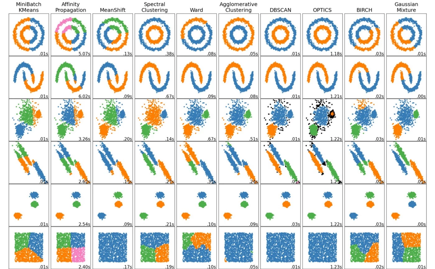
In this article, you will find a complete clustering cheat sheet. In eleven minutes you will be able to know what it is and to refresh your memory of the main algorithms.
Clustering (also called cluster analysis) is a task of grouping similar instances into clusters. More formally, clustering is the task of grouping the population of unlabeled data points into clusters in a way that data points in the same cluster are more similar to each other than to data points in other clusters.
The clustering task is probably the most important in unsupervised learning, since it has many applications, for example:
- data analysis: often a huge dataset contains several large clusters, analyzing which separately, you can come to interesting insights;
- anomaly detection: as we saw before, data points located in the regions of low density can be considered as anomalies;
- semi-supervised learning: clustering approaches often helps you to automatically label partially labeled data for classification tasks;
- indirectly clustering tasks (tasks where clustering helps to gain good results): recommender systems, search engines, etc., and
- directly clustering tasks: customer segmentation, image segmentation, etc.
All clustering algorithms require data preprocessing and standardization. Most clustering algorithms perform worse with a large number of features, so it is sometimes recommended to use methods of dimensionality reduction before clustering.
K-Means
K-Means algorithm is based on the centroid concept. Centroid is a geometric center of a cluster (mean of coordinates of all cluster points). First, centroids are initialized randomly (this is the basic option, but there are other initialization techniques). After that, we iteratively do the two following steps, while centroids are moving:
- Update the clusters — for each data point assign it a cluster number with the nearest centroid, and
- Update the clusters’ centroids — calculate the new mean value of the cluster elements to move centroids.
The strengths and weaknesses of the algorithm are intuitive. It is simple and fast, but it requires initial knowledge about the number of clusters. It also does not detect clusters of complex shapes well and can result in a local solution. To choose a good number of clusters we can use a sum of squared distances from data points to cluster centroids as a metric and choose the number when this metric stops falling fast (elbow method). To find a globally optimal solution, you can run the algorithm several times and choose the best result (n_init parameter in sklearn).
A speeded version of this algorithm is Mini Batch K-Means. In that case, we use a random subsample instead of the whole dataset for calculations. There are a lot of other modifications, and many of them are implemented in sklearn.
Pros:
- Simple and intuitive;
- Scales to large datasets;
- As a result, we also have centroids that can be used as standard cluster representatives.
Cons:
- Knowledge about the number of clusters is necessary and must be specified as a parameter;
- Does not cope well with a very large number of features;
- Separates only convex and homogeneous clusters well;
- Can result in poor local solutions, so it needs to be run several times.
Hierarchical Clustering
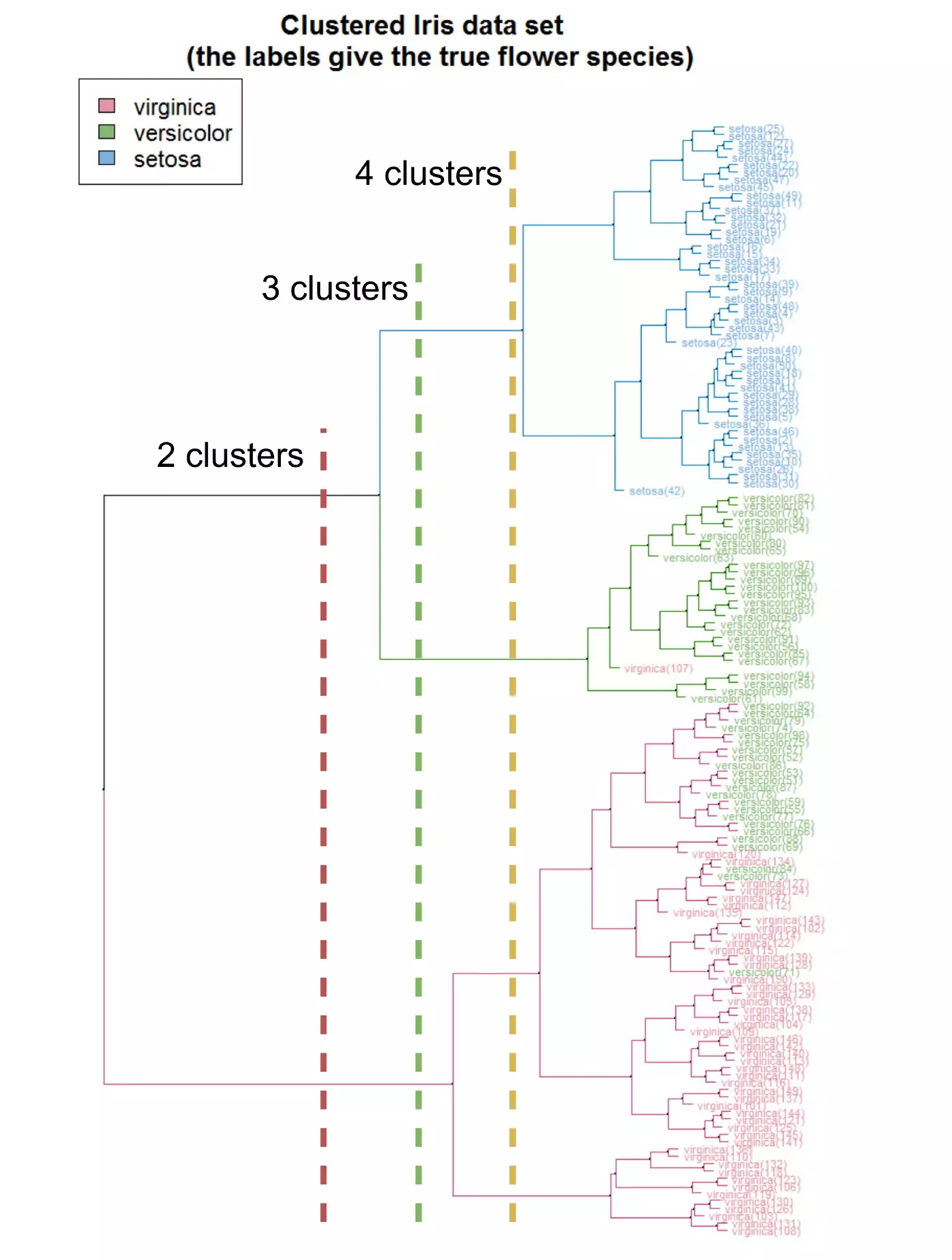
Hierarchical clustering (also Hierarchical Cluster Analysis (HCA) or Agglomerative Clustering) is a family of clustering algorithms that build a hierarchy of clusters during the analysis.
It is represented as a dendrogram (a tree diagram). The root of the tree (usually the upper or left element) is one large cluster that contains all data points. The leaves (bottom or right elements) are tiny clusters, each of which contains only one data point. According to the generated dendrogram, you can choose the desired separation into any number of clusters.
This family of algorithms requires calculating the distance between clusters. Different metrics are used for this purpose (simple linkage, complete linkage, average linkage, centroid linkage, etc.), but one of the most effective and popular is Ward’s distance or Ward’s linkage.
To learn more about the different methods of measuring the distance between clusters, start with this article.
Pros:
- Simple and intuitive;
- Works well when data has a hierarchical structure.
- Knowledge about the number of clusters is not necessary.
Cons:
- Requires additional analysis to choose the resulting number of clusters;
- Separates only convex and homogeneous clusters well;
- A greedy algorithm can result in poor local solutions.
Spectral Clustering
The spectral clustering approach is based on graph theory and linear algebra. This algorithm uses the spectrum (set of eigenvalues) of the similarity matrix (that contains the similarity of each pair of data points) to perform dimensionality reduction. Then it uses some of the clustering algorithms in this low-dimensional space (sklearn.cluster.SpectralClustering class uses K-Means).
Due to the dimensionality reduction, this algorithm can detect complex cluster structures and shapes. It can also be used to search for clusters in graphs. However, due to its computational complexity, it does not work well with large datasets.
Pros:
- Can detect complex cluster structures and shapes;
- Can be used to search for clusters in graphs.
Cons:
- Knowledge about the number of clusters is necessary and must be specified as a parameter;
- Does not cope well with a very large number of instances;
- Does not cope well when the clusters have very different sizes.
DBSCAN
The DBSCAN abbreviation stands for Density-Based Spatial Clustering of Applications with Noise.
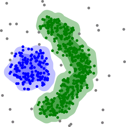
According to this algorithm, clusters are high-density regions (where the data points are located close to each other) separated by low-density regions (where the data points are located far from each other).
The central concept of the DBSCAN algorithm is the idea of a core sample, which means a sample located in an area of high density. Data point A is considered a core sample if at least min_samples other instances (usually including A) are located within eps distance from A.
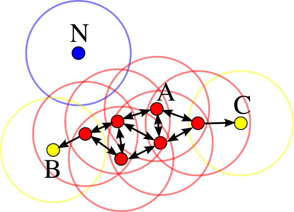
Therefore, a cluster is a group of core samples located close to each other and some non-core samples located close to core samples. Other samples are defined as outliers (or anomalies) and do not belong to any cluster. This approach is called density-based clustering. It allows you not to specify the number of clusters as a parameter and find clusters of complex shapes.
An extension or generalization of the DBSCAN algorithm is the OPTICS algorithm (Ordering Points To Identify the Clustering Structure).
Pros:
- Knowledge about the number of clusters is not necessary;
- Also solves the anomaly detection task.
Cons:
- Need to select and tune the density parameter (eps);
- Does not cope well with sparse data.
Affinity Propagation
The Affinity Propagation algorithm also does not require knowledge about the number of clusters. But unlike DBSCAN, which is a density-based clustering algorithm, affinity propagation is based on the idea of passing messages between data points. Calculating pairwise similarity based on some distance function (i.e. Euclidean distance) this algorithm then converges in some number of standard representatives. A dataset is then described using this small number of standard representatives, which are identified as the most representative instances on the particular cluster.
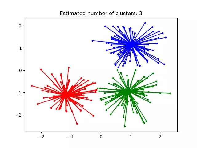
The results of this algorithm often leave much to be desired, but it has a number of strong advantages. However, its main disadvantage, the computational complexity (caused by the need to calculate the distance for all possible pairs of data points) does not allow it to be used on large datasets.
Pros:
- Knowledge about the number of clusters is not necessary;
- As a result, we also have standard representatives of a cluster.
- Unlike K-Means centroids, these instances are not just average values, but real objects from the dataset.
Cons:
- Works much slower than other algorithms due to computational complexity;
- Does not cope well with a large number of instances;
- Separates only convex and homogeneous clusters well.
Mean Shift
The Mean Shift algorithm first places a circle of a certain size (radius of the circle is a parameter called bandwidth) in the center of each data point. After that, it iteratively calculates the mean for each circle (the average coordinates among the points inside the circle) and shifts it. These mean-shift steps are performed until the algorithm converges and the circles stop moving.
You can see Mean Shift algorithm visualization here.
Mean Shift converges into local regions with maximum density. Then all the circles that are close enough to each other form a cluster. Therefore, at the same time, it solves the density estimation task and calculates cluster centroids.
As DBSCAN, this algorithm represents a density-based approach so works badly with sparse data.
Pros:
- Knowledge about the number of clusters is not necessary;
- Have just one hyperparameter: the radius of the circles;
- Solves density estimation task and calculate cluster centroids;
Cons:
- Does not find a cluster structure where it is not actually present.
- Does not cope well with sparse data and with a large number of features;
- Does not cope well with a large number of instances;
- Does not cope well with clusters of complex shapes: tends to chop these clusters into pieces.
BIRCH
The BIRCH stands for Balanced Iterative Reducing and Clustering using Hierarchies.
This hierarchical clustering algorithm was designed specifically for large datasets. In the majority of cases, it has a computational complexity of $O(n)$, so requires only one scan of the dataset.
During training, it creates a dendrogram containing enough information to quickly assign each new data instance to some cluster without having to store information about all instances in memory. These principles allow getting the best quality for a given set of memory and time resources compared with other clustering algorithms. They also allow to incrementally cluster incoming data instances performing online learning.
Pros:
- Was designed specifically for very large datasets;
- Show the best quality for a given set of memory and time resources;
- Allows implementing online clustering.
Cons:
- Does not cope well with a large number of features.
Gaussian Mixture Models
Gaussian Mixture Models (GMM) is a probabilistic algorithm that can solve as many as three unsupervised learning tasks: clustering, density estimation, and anomaly detection.
This method is based on the Expectation Maximization algorithm and assumes that data points were generated from a group (mixture) of Gaussian distributions. This algorithm can result in poor local solutions, so it needs to be run several times keeping only the best solution (n_init parameter in sklearn).
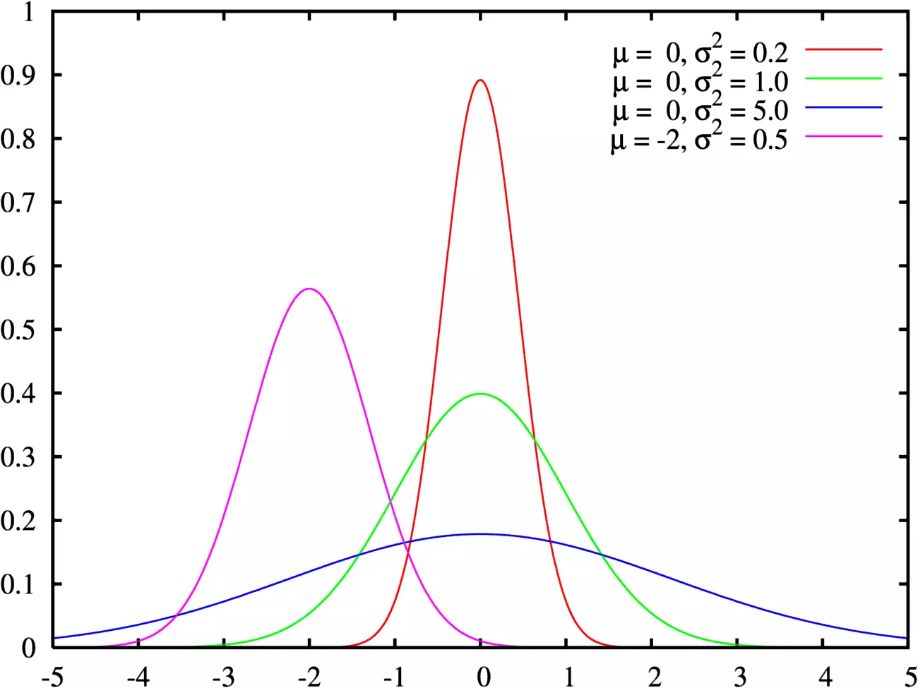
It is known that in the general case the Gaussian distribution has two parameters: a vector of the mean $\mu$ and a matrix of variance $\sigma^{2}$. Then, if it is known that the data can be divided into N clusters in M-dimensional space, the task of the algorithm is to select $N\mu$ vectors (with M elements) and $N\sigma^{2}$ matrices (with MxM elements).
In the case of one-dimensional space, both $\mu$ and $\sigma^{2}$ are scalars (single numbers).
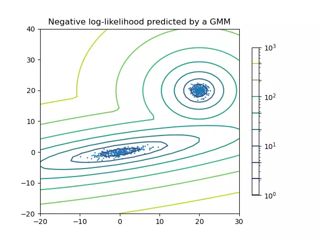
In the image below you can see two distributions in two-dimensional space. Each of the distributions has the following parameters:
- two values for the mean vectors (x and y coordinates);
- four values for the variance matrices (variances in main diagonal and covariances in the other elements).
To choose a good number of clusters you can use BIC or AIC (Bayesian / Akaike information criterion) as metrics and choose the model with its minimum value. On the other hand, you can use the Bayesian GMM algorithm. This model only requires a value that is greater than the possible number of clusters and can detect the optimal number itself.
Also, the Gaussian Mixture Model is a generative model, meaning that you can sample new instances from it. It is also possible to estimate the density of the model at any given location.
Pros:
- Perfectly deals with datasets that were generated from a mixture of Gaussian distributions with different shapes and sizes;
- At the same time solves density estimation and anomaly detection tasks;
- Is a generative model, so can generate new instances.
Cons:
- Knowledge about the number of clusters is necessary and must be specified as a parameter (not in the case of Bayesian GMM);
- Expectation Maximization algorithm can result in poor local solutions, so it needs to be run several times;
- Does not scale well with large numbers of features;
- Assume that data instances were generated from a mixture of Gaussian distributions, so cope badly with data of other shapes.
How to choose a clustering algorithm?
As you can see, the clustering task is quite difficult and have a wide variety of applications, so it’s almost impossible to build some universal set of rules to select a clustering algorithm — all of them have advantages and disadvantages.
Things become better when you have some assumptions about your data, so data analysis can help you with that. What is the approximate number of clusters? Are they located far from each other or do they intersect? Are they similar in shape and density? All that information can help you to solve your task better.
If the number of clusters is unknown, a good initial approximation is the square root of the number of objects. You can also first run an algorithm that does not require a number of clusters as a parameter (DBSCAN or Affinity Propagation) and use the resulting value as a starting point.
Another important question remains the evaluation of quality — you can try all the algorithms, but how to decide which one is the best? There are a great many metrics for this — from homogeneity and completeness to silhouette — they show themselves differently in different tasks. Understanding these metrics and how to use them successfully comes with experience and goes beyond the scope of this article.
Nevertheless, I managed to list and review all the main clustering algorithms and approaches. Hope this will help you and motivate you to dive deeper into cluster analysis.
You may also be interested in: