The Convolutional Classifier
Have you ever wanted to teach a computer to see?
Here, we will:
- Use modern deep-learning networks to build an image classifier with Keras.
- Design your own custom convnet with reusable blocks.
- Learn the fundamental ideas behind visual feature extraction.
- Master the art of transfer learning to boost your models.
- Utilize data augmentation to extend your dataset.
Introduction
This series will introduce you to the fundamental ideas of computer vision. Our goal is to learn how a neural network can “understand” a natural image well-enough to solve the same kinds of problems the human visual system can solve.
The neural networks that are best at this task are called convolutional neural networks (Sometimes we say convnet or CNN instead.) Convolution is the mathematical operation that gives the layers of a convnet their unique structure. In future lessons, you’ll learn why this structure is so effective at solving computer vision problems.
We will apply these ideas to the problem of image classification: given a picture, can we train a computer to tell us what it’s a picture of? You may have seen apps that can identify a species of plant from a photograph. That’s an image classifier! In this course, you’ll learn how to build image classifiers just as powerful as those used in professional applications.
While our focus will be on image classification, what you’ll learn in this course is relevant to every kind of computer vision problem. At the end, you’ll be ready to move on to more advanced applications like generative adversarial networks and image segmentation.
The Convolutional Classifier
A convnet used for image classification consists of two parts: a convolutional base and a dense head.
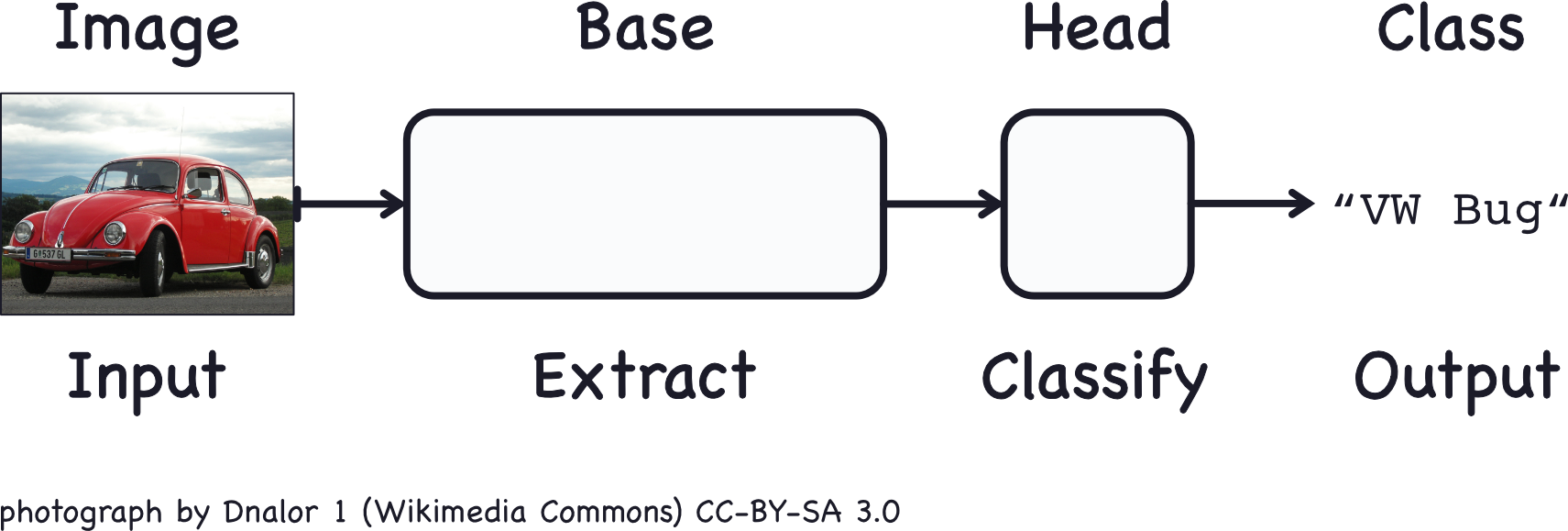
The base is used to extract the features from an image. It is formed primarily of layers performing the convolution operation, but often includes other kinds of layers as well.
The head is used to determine the class of the image. It is formed primarily of dense layers, but might include other layers like dropout.
What do we mean by visual feature? A feature could be a line, a color, a texture, a shape, a pattern – or some complicated combination.
The whole process goes something like this:
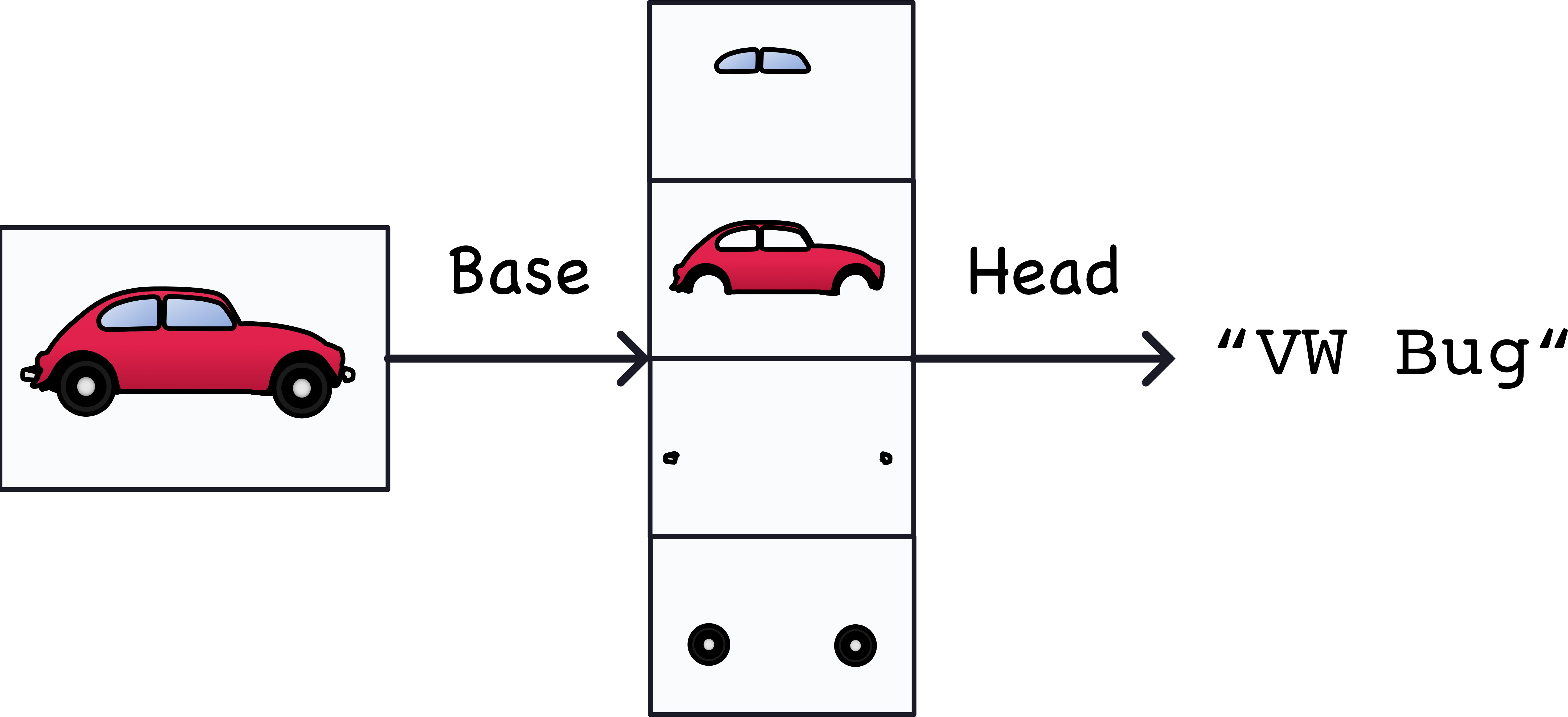
The features actually extracted look a bit different, but it gives the idea.
Training the Classifier
The goal of the network during training is to learn two things:
- Which features to extract from an image (base),
- Which class goes with what features (head).
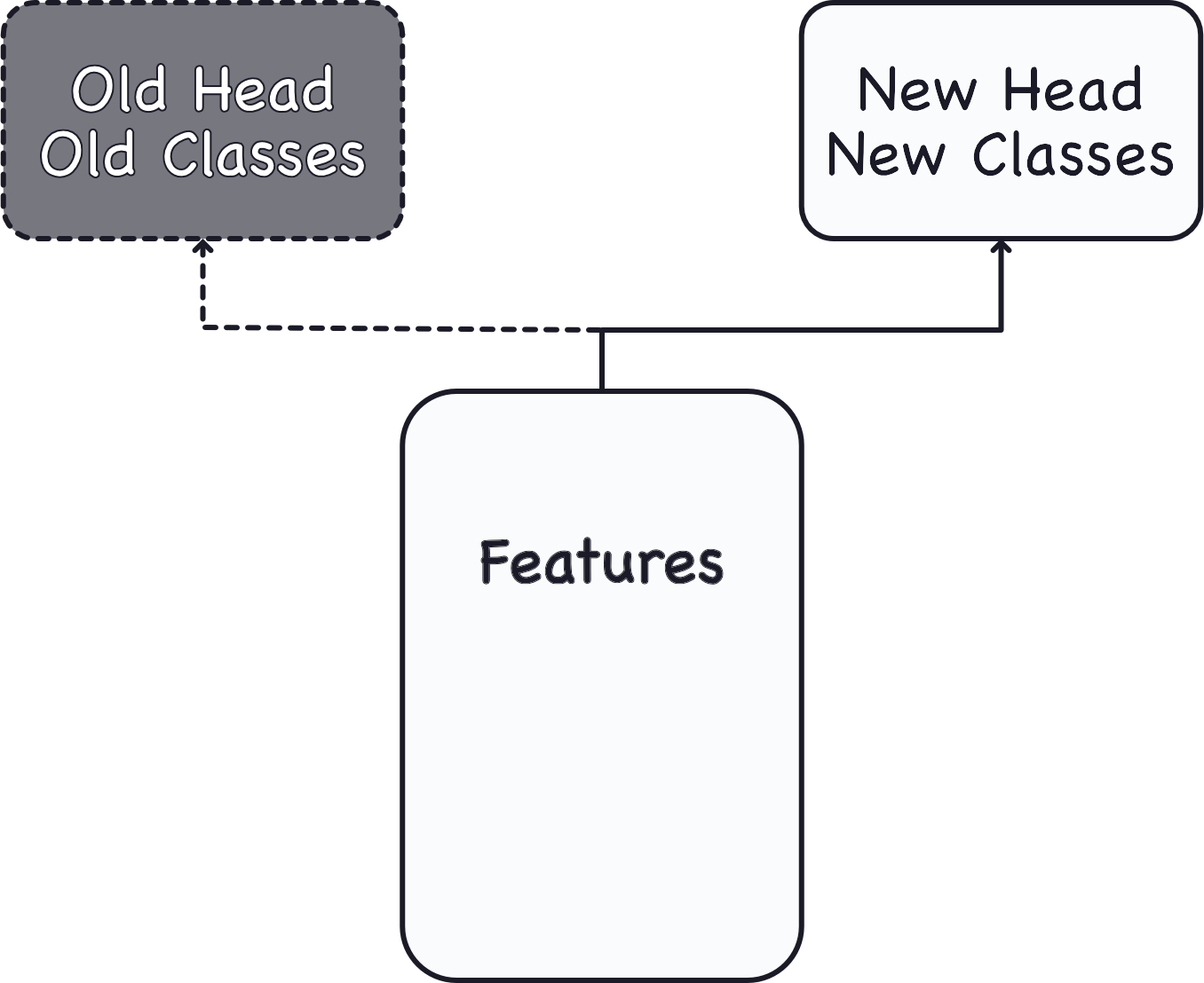
These days, convnets are rarely trained from scratch. More often, we reuse the base of a pretrained model. To the pretrained base we then attach an untrained head. In other words, we reuse the part of a network that has already learned to do 1. Extract features, and attach to it some fresh layers to learn 2. Classify.
Example - Train a Convnet Classifier
We’re going to be creating classifiers that attempt to solve the following problem: is this a picture of a Car or of a Truck? Our dataset is about 10,000 pictures of various automobiles, around half cars and half trucks.
Steps:
- Load Data
- Define Pretrained Base
- Attach Head
- Train
# Imports
import os, warnings
import matplotlib.pyplot as plt
from matplotlib import gridspec
import matplotlib.pyplot as plt

import numpy as np
import tensorflow as tf
from tensorflow.keras.preprocessing import image_dataset_from_directory

# Reproducability
def set_seed(seed=31415):
    np.random.seed(seed)
    tf.random.set_seed(seed)
    os.environ['PYTHONHASHSEED'] = str(seed)
    os.environ['TF_DETERMINISTIC_OPS'] = '1'
set_seed(31415)

# Set Matplotlib defaults
plt.rc('figure', autolayout=True)
plt.rc('axes', labelweight='bold', labelsize='large',
       titleweight='bold', titlesize=18, titlepad=10)
plt.rc('image', cmap='magma')
warnings.filterwarnings("ignore") # to clean up output cells


# Load training and validation sets
ds_train_ = image_dataset_from_directory(
    '../input/car-or-truck/train',
    labels='inferred',
    label_mode='binary',
    image_size=[128, 128],
    interpolation='nearest',
    batch_size=64,
    shuffle=True,
)
ds_valid_ = image_dataset_from_directory(
    '../input/car-or-truck/valid',
    labels='inferred',
    label_mode='binary',
    image_size=[128, 128],
    interpolation='nearest',
    batch_size=64,
    shuffle=False,
)

# Data Pipeline
def convert_to_float(image, label):
    image = tf.image.convert_image_dtype(image, dtype=tf.float32)
    return image, label

AUTOTUNE = tf.data.experimental.AUTOTUNE
ds_train = (
    ds_train_
    .map(convert_to_float)
    .cache()
    .prefetch(buffer_size=AUTOTUNE)
)
ds_valid = (
    ds_valid_
    .map(convert_to_float)
    .cache()
    .prefetch(buffer_size=AUTOTUNE)
)
Found 5117 files belonging to 2 classes.
2021-11-09 00:11:56.193766: I tensorflow/stream_executor/cuda/cuda_gpu_executor.cc:937] successful NUMA node read from SysFS had negative value (-1), but there must be at least one NUMA node, so returning NUMA node zero
2021-11-09 00:11:56.297337: I tensorflow/stream_executor/cuda/cuda_gpu_executor.cc:937] successful NUMA node read from SysFS had negative value (-1), but there must be at least one NUMA node, so returning NUMA node zero
2021-11-09 00:11:56.298014: I tensorflow/stream_executor/cuda/cuda_gpu_executor.cc:937] successful NUMA node read from SysFS had negative value (-1), but there must be at least one NUMA node, so returning NUMA node zero
2021-11-09 00:11:56.307670: I tensorflow/core/platform/cpu_feature_guard.cc:142] This TensorFlow binary is optimized with oneAPI Deep Neural Network Library (oneDNN) to use the following CPU instructions in performance-critical operations:  AVX2 AVX512F FMA
To enable them in other operations, rebuild TensorFlow with the appropriate compiler flags.
2021-11-09 00:11:56.308421: I tensorflow/stream_executor/cuda/cuda_gpu_executor.cc:937] successful NUMA node read from SysFS had negative value (-1), but there must be at least one NUMA node, so returning NUMA node zero
2021-11-09 00:11:56.309104: I tensorflow/stream_executor/cuda/cuda_gpu_executor.cc:937] successful NUMA node read from SysFS had negative value (-1), but there must be at least one NUMA node, so returning NUMA node zero
2021-11-09 00:11:56.309707: I tensorflow/stream_executor/cuda/cuda_gpu_executor.cc:937] successful NUMA node read from SysFS had negative value (-1), but there must be at least one NUMA node, so returning NUMA node zero
2021-11-09 00:11:58.119581: I tensorflow/stream_executor/cuda/cuda_gpu_executor.cc:937] successful NUMA node read from SysFS had negative value (-1), but there must be at least one NUMA node, so returning NUMA node zero
2021-11-09 00:11:58.120396: I tensorflow/stream_executor/cuda/cuda_gpu_executor.cc:937] successful NUMA node read from SysFS had negative value (-1), but there must be at least one NUMA node, so returning NUMA node zero
2021-11-09 00:11:58.121067: I tensorflow/stream_executor/cuda/cuda_gpu_executor.cc:937] successful NUMA node read from SysFS had negative value (-1), but there must be at least one NUMA node, so returning NUMA node zero
2021-11-09 00:11:58.121644: I tensorflow/core/common_runtime/gpu/gpu_device.cc:1510] Created device /job:localhost/replica:0/task:0/device:GPU:0 with 15403 MB memory:  -> device: 0, name: Tesla P100-PCIE-16GB, pci bus id: 0000:00:04.0, compute capability: 6.0
Found 5051 files belonging to 2 classes.
The most commonly used dataset for pretraining is ImageNet, a large dataset of many kind of natural images. Keras includes a variety models pretrained on ImageNet in its applications module. The pretrained model we’ll use is called VGG16.
pretrained_base = tf.keras.models.load_model(
    '../input/cv-course-models/cv-course-models/vgg16-pretrained-base',
)
pretrained_base.trainable = False
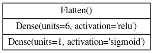
Next, we attach the classifier head. For this example, we’ll use a layer of hidden units (the first Dense layer) followed by a layer to transform the outputs to a probability score for class 1, Truck. The Flatten layer transforms the two dimensional outputs of the base into the one dimensional inputs needed by the head.
from tensorflow import keras
from tensorflow.keras import layers

model = keras.Sequential([
    pretrained_base,
    layers.Flatten(),
    layers.Dense(6, activation='relu'),
    layers.Dense(1, activation='sigmoid'),
])
Finally, let’s train the model. Since this is a two-class problem, we’ll use the binary versions of cross entropy and accuracy. The adam optimizer generally performs well, so we’ll choose it as well.
model.compile(
    optimizer='adam',
    loss='binary_crossentropy',
    metrics=['binary_accuracy'],
)

history = model.fit(
    ds_train,
    validation_data=ds_valid,
    epochs=30,
    verbose=0,
)
2021-11-09 00:12:03.591628: I tensorflow/compiler/mlir/mlir_graph_optimization_pass.cc:185] None of the MLIR Optimization Passes are enabled (registered 2)
2021-11-09 00:12:06.918477: I tensorflow/stream_executor/cuda/cuda_dnn.cc:369] Loaded cuDNN version 8005
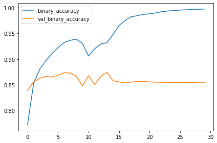
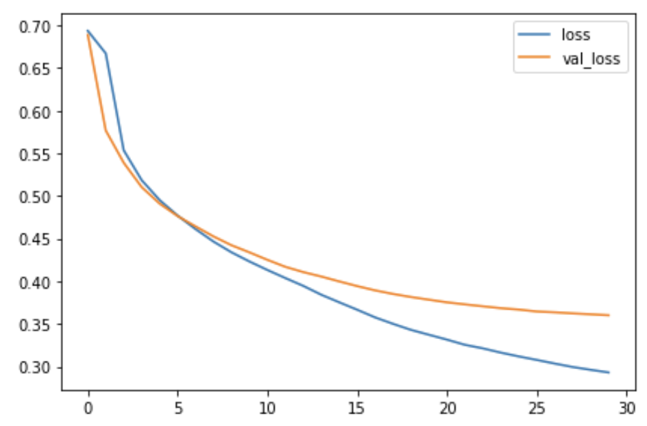
When training a neural network, it’s always a good idea to examine the loss and metric plots. The history object contains this information in a dictionary history.history. We can use Pandas to convert this dictionary to a dataframe and plot it with a built-in method.
import pandas as pd

history_frame = pd.DataFrame(history.history)
history_frame.loc[:, ['loss', 'val_loss']].plot()
history_frame.loc[:, ['binary_accuracy', 'val_binary_accuracy']].plot();
Conclusion
In this lesson, we learned about the structure of a convnet classifier: a head to act as a classifier atop of a base which performs the feature extraction.
The head, essentially, is an ordinary classifier like you learned about in the introductory course. For features, it uses those features extracted by the base. This is the basic idea behind convolutional classifiers: that we can attach a unit that performs feature engineering to the classifier itself.
This is one of the big advantages deep neural networks have over traditional machine learning models: given the right network structure, the deep neural net can learn how to engineer the features it needs to solve its problem.
Example - InceptionV1
In the tutorial, we saw how to build an image classifier by attaching a head of dense layers to a pretrained base. The base we used was from a model called VGG16. We saw that the VGG16 architecture was prone to overfitting this dataset. Over this course, you’ll learn a number of ways you can improve upon this initial attempt.
The first way you’ll see is to use a base more appropriate to the dataset. The base this model comes from is called InceptionV1 (also known as GoogLeNet). InceptionV1 was one of the early winners of the ImageNet competition. One of its successors, InceptionV4, is among the state of the art today.
# Imports
import os, warnings
import matplotlib.pyplot as plt
from matplotlib import gridspec

import numpy as np
import tensorflow as tf
from tensorflow.keras.preprocessing import image_dataset_from_directory

# Reproducability
def set_seed(seed=31415):
    np.random.seed(seed)
    tf.random.set_seed(seed)
    os.environ['PYTHONHASHSEED'] = str(seed)
    os.environ['TF_DETERMINISTIC_OPS'] = '1'
set_seed()

# Set Matplotlib defaults
plt.rc('figure', autolayout=True)
plt.rc('axes', labelweight='bold', labelsize='large',
       titleweight='bold', titlesize=18, titlepad=10)
plt.rc('image', cmap='magma')
warnings.filterwarnings("ignore") # to clean up output cells


# Load training and validation sets
ds_train_ = image_dataset_from_directory(
    '../input/car-or-truck/train',
    labels='inferred',
    label_mode='binary',
    image_size=[128, 128],
    interpolation='nearest',
    batch_size=64,
    shuffle=True,
)
ds_valid_ = image_dataset_from_directory(
    '../input/car-or-truck/valid',
    labels='inferred',
    label_mode='binary',
    image_size=[128, 128],
    interpolation='nearest',
    batch_size=64,
    shuffle=False,
)

# Data Pipeline
def convert_to_float(image, label):
    image = tf.image.convert_image_dtype(image, dtype=tf.float32)
    return image, label

AUTOTUNE = tf.data.experimental.AUTOTUNE
ds_train = (
    ds_train_
    .map(convert_to_float)
    .cache()
    .prefetch(buffer_size=AUTOTUNE)
)
ds_valid = (
    ds_valid_
    .map(convert_to_float)
    .cache()
    .prefetch(buffer_size=AUTOTUNE)
)
The InceptionV1 model pretrained on ImageNet is available in the TensorFlow Hub repository, but we’ll load it from a local copy. Run this cell to load InceptionV1 for your base.
import tensorflow_hub as hub

pretrained_base = tf.keras.models.load_model(
    '../input/cv-course-models/cv-course-models/inceptionv1'
)
Define Pretrained Base
Now that you have a pretrained base to do our feature extraction, decide whether this base should be trainable or not.
pretrained_base.trainable = False
When doing transfer learning, it’s generally not a good idea to retrain the entire base – at least not without some care. The reason is that the random weights in the head will initially create large gradient updates, which propogate back into the base layers and destroy much of the pretraining. Using techniques known as fine tuning it’s possible to further train the base on new data, but this requires some care to do well.
Attach Head
Now that the base is defined to do the feature extraction, create a head of Dense layers to perform the classification, following this diagram:
from tensorflow import keras
from tensorflow.keras import layers

model = keras.Sequential([
    pretrained_base,
    layers.Flatten(),
    layers.Dense(6, activation='relu'),
    layers.Dense(1, activation='sigmoid'),
])
Train
Before training a model in Keras, you need to specify an optimizer to perform the gradient descent, a loss function to be minimized, and (optionally) any performance metrics. The optimization algorithm we’ll use for this course is called “Adam”, which generally performs well regardless of what kind of problem you’re trying to solve.
The loss and the metrics, however, need to match the kind of problem you’re trying to solve. Our problem is a binary classification problem: Car coded as 0, and Truck coded as 1. Choose an appropriate loss and an appropriate accuracy metric for binary classification.
optimizer = tf.keras.optimizers.Adam(epsilon=0.01)
model.compile(
    optimizer='adam',
    loss='binary_crossentropy',
    metrics=['binary_accuracy'],
)
history = model.fit(
    ds_train,
    validation_data=ds_valid,
    epochs=30,
)
Epoch 1/30
80/80 [==============================] - ETA: 0s - loss: 0.6936 - binary_accuracy: 0.5706
import pandas as pd
history_frame = pd.DataFrame(history.history)
history_frame.loc[:, ['loss', 'val_loss']].plot()
history_frame.loc[:, ['binary_accuracy', 'val_binary_accuracy']].plot();
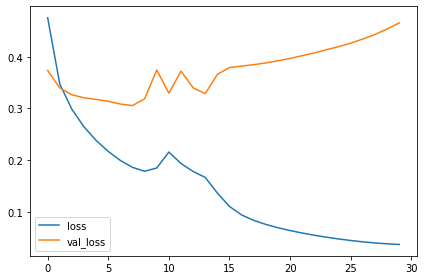
Examine Loss and Accuracy
Do you notice a difference between these learning curves and the curves for VGG16 from the tutorial? What does this difference tell you about what this model (InceptionV2) learned compared to VGG16? Are there ways in which one is better than the other? Worse?
That the training loss and validation loss stay fairly close is evidence that the model isn’t just memorizing the training data, but rather learning general properties of the two classes. But, because this model converges at a loss greater than the VGG16 model, it’s likely that it is underfitting some, and could benefit from some extra capacity.
Conclusion
In this first lesson, you learned the basics of convolutional image classifiers, that they consist of a base for extracting features from images, and a head which uses the features to decide the image’s class. You also saw how to build a classifier with transfer learning on pretrained base.