Custom Convnets

Now that you’ve seen the layers a convnet uses to extract features, it’s time to put them together and build a network of your own!

Simple to Refined

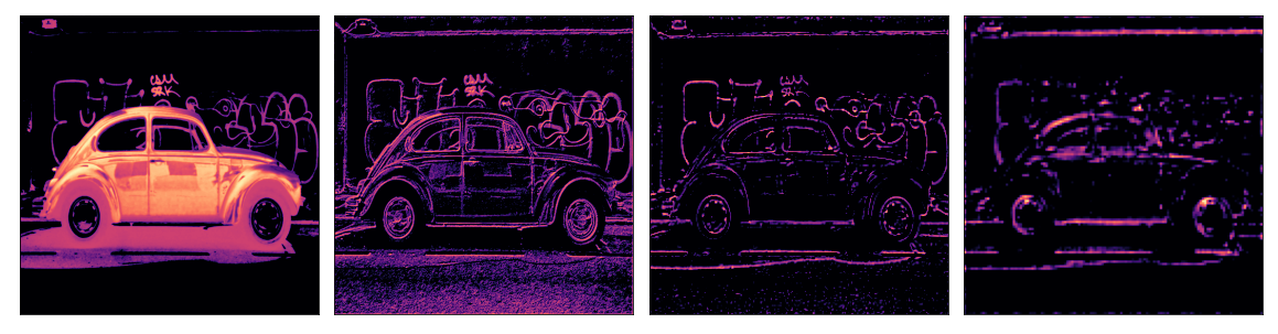
In the last three lessons, we saw how convolutional networks perform feature extraction through three operations: filter, detect, and condense. A single round of feature extraction can only extract relatively simple features from an image, things like simple lines or contrasts. These are too simple to solve most classification problems. Instead, convnets will repeat this extraction over and over, so that the features become more complex and refined as they travel deeper into the network.

Convolutional Blocks

It does this by passing them through long chains of convolutional blocks which perform this extraction.

These convolutional blocks are stacks of Conv2D and MaxPool2D layers.

Each block represents a round of extraction, and by composing these blocks the convnet can combine and recombine the features produced, growing them and shaping them to better fit the problem at hand. The deep structure of modern convnets is what allows this sophisticated feature engineering and has been largely responsible for their superior performance.

Example - Design a Convnet

Let’s see how to define a deep convolutional network capable of engineering complex features. In this example, we’ll create a Keras Sequence model and then train it on our Cars dataset.

# Imports
import os, warnings
import matplotlib.pyplot as plt
from matplotlib import gridspec

import numpy as np
import tensorflow as tf
from tensorflow.keras.preprocessing import image_dataset_from_directory

# Reproducability
def set_seed(seed=31415):
    np.random.seed(seed)
    tf.random.set_seed(seed)
    os.environ['PYTHONHASHSEED'] = str(seed)
    os.environ['TF_DETERMINISTIC_OPS'] = '1'
set_seed()

# Set Matplotlib defaults
plt.rc('figure', autolayout=True)
plt.rc('axes', labelweight='bold', labelsize='large',
       titleweight='bold', titlesize=18, titlepad=10)
plt.rc('image', cmap='magma')
warnings.filterwarnings("ignore") # to clean up output cells


# Load training and validation sets
ds_train_ = image_dataset_from_directory(
    '../input/car-or-truck/train',
    labels='inferred',
    label_mode='binary',
    image_size=[128, 128],
    interpolation='nearest',
    batch_size=64,
    shuffle=True,
)
ds_valid_ = image_dataset_from_directory(
    '../input/car-or-truck/valid',
    labels='inferred',
    label_mode='binary',
    image_size=[128, 128],
    interpolation='nearest',
    batch_size=64,
    shuffle=False,
)

# Data Pipeline
def convert_to_float(image, label):
    image = tf.image.convert_image_dtype(image, dtype=tf.float32)
    return image, label

AUTOTUNE = tf.data.experimental.AUTOTUNE
ds_train = (
    ds_train_
    .map(convert_to_float)
    .cache()
    .prefetch(buffer_size=AUTOTUNE)
)
ds_valid = (
    ds_valid_
    .map(convert_to_float)
    .cache()
    .prefetch(buffer_size=AUTOTUNE)
)

Define Model

Here is a diagram of the model we’ll use:

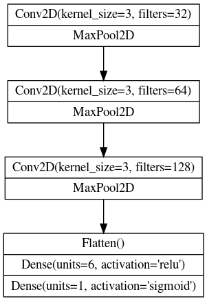
Now we’ll define the model. See how our model consists of three blocks of Conv2D and MaxPool2D layers (the base) followed by a head of Dense layers. We can translate this diagram more or less directly into a Keras Sequential model just by filling in the appropriate parameters.

from tensorflow import keras
from tensorflow.keras import layers

model = keras.Sequential([

    # First Convolutional Block
    layers.Conv2D(filters=32, kernel_size=5, activation="relu", padding='same',
                  # give the input dimensions in the first layer
                  # [height, width, color channels(RGB)]
                  input_shape=[128, 128, 3]),
    layers.MaxPool2D(),

    # Second Convolutional Block
    layers.Conv2D(filters=64, kernel_size=3, activation="relu", padding='same'),
    layers.MaxPool2D(),

    # Third Convolutional Block
    layers.Conv2D(filters=128, kernel_size=3, activation="relu", padding='same'),
    layers.MaxPool2D(),

    # Classifier Head
    layers.Flatten(),
    layers.Dense(units=6, activation="relu"),
    layers.Dense(units=1, activation="sigmoid"),
])
model.summary()

Model: "sequential"
_________________________________________________________________
Layer (type)                 Output Shape              Param #   
=================================================================
conv2d (Conv2D)              (None, 128, 128, 32)      2432      
_________________________________________________________________
max_pooling2d (MaxPooling2D) (None, 64, 64, 32)        0         
_________________________________________________________________
conv2d_1 (Conv2D)            (None, 64, 64, 64)        18496     
_________________________________________________________________
max_pooling2d_1 (MaxPooling2 (None, 32, 32, 64)        0         
_________________________________________________________________
conv2d_2 (Conv2D)            (None, 32, 32, 128)       73856     
_________________________________________________________________
max_pooling2d_2 (MaxPooling2 (None, 16, 16, 128)       0         
_________________________________________________________________
flatten (Flatten)            (None, 32768)             0         
_________________________________________________________________
dense (Dense)                (None, 6)                 196614    
_________________________________________________________________
dense_1 (Dense)              (None, 1)                 7         
=================================================================
Total params: 291,405
Trainable params: 291,405
Non-trainable params: 0
_________________________________________________________________

Notice in this definition is how the number of filters doubled block-by-block: $64, 128, 256$. This is a common pattern. Since the MaxPool2D layer is reducing the size of the feature maps, we can afford to increase the quantity we create.

Train

model.compile(
    optimizer=tf.keras.optimizers.Adam(epsilon=0.01),
    loss='binary_crossentropy',
    metrics=['binary_accuracy']
)

history = model.fit(
    ds_train,
    validation_data=ds_valid,
    epochs=40,
    verbose=0,
)

import pandas as pd

history_frame = pd.DataFrame(history.history)
history_frame.loc[:, ['loss', 'val_loss']].plot()
history_frame.loc[:, ['binary_accuracy', 'val_binary_accuracy']].plot();

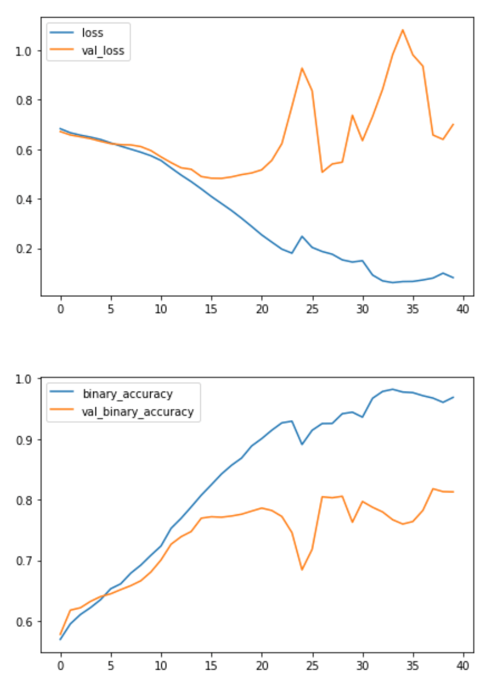
This model is much smaller than the VGG16 model from Lesson 1 – only 3 convolutional layers versus the 16 of VGG16. It was nevertheless able to fit this dataset fairly well. We might still be able to improve this simple model by adding more convolutional layers, hoping to create features better adapted to the dataset.

---

Exercise

In these exercises, you’ll build a custom convnet with performance competitive to the VGG16 model from Lesson 1.

# Imports
import os, warnings
import matplotlib.pyplot as plt
from matplotlib import gridspec

import numpy as np
import tensorflow as tf
from tensorflow.keras.preprocessing import image_dataset_from_directory

# Reproducability
def set_seed(seed=31415):
    np.random.seed(seed)
    tf.random.set_seed(seed)
    os.environ['PYTHONHASHSEED'] = str(seed)
    os.environ['TF_DETERMINISTIC_OPS'] = '1'
set_seed()

# Set Matplotlib defaults
plt.rc('figure', autolayout=True)
plt.rc('axes', labelweight='bold', labelsize='large',
       titleweight='bold', titlesize=18, titlepad=10)
plt.rc('image', cmap='magma')
warnings.filterwarnings("ignore") # to clean up output cells


# Load training and validation sets
ds_train_ = image_dataset_from_directory(
    '../input/car-or-truck/train',
    labels='inferred',
    label_mode='binary',
    image_size=[128, 128],
    interpolation='nearest',
    batch_size=64,
    shuffle=True,
)
ds_valid_ = image_dataset_from_directory(
    '../input/car-or-truck/valid',
    labels='inferred',
    label_mode='binary',
    image_size=[128, 128],
    interpolation='nearest',
    batch_size=64,
    shuffle=False,
)

# Data Pipeline
def convert_to_float(image, label):
    image = tf.image.convert_image_dtype(image, dtype=tf.float32)
    return image, label

AUTOTUNE = tf.data.experimental.AUTOTUNE
ds_train = (
    ds_train_
    .map(convert_to_float)
    .cache()
    .prefetch(buffer_size=AUTOTUNE)
)
ds_valid = (
    ds_valid_
    .map(convert_to_float)
    .cache()
    .prefetch(buffer_size=AUTOTUNE)
)

Design a Convnet

Let’s design a convolutional network with a block architecture like we saw in the tutorial. The model from the example had three blocks, each with a single convolutional layer. Its performance on the “Car or Truck” problem was okay, but far from what the pretrained VGG16 could achieve. It might be that our simple network lacks the ability to extract sufficiently complex features. We could try improving the model either by adding more blocks or by adding convolutions to the blocks we have.

Let’s go with the second approach. We’ll keep the three block structure, but increase the number of Conv2D layer in the second block to two, and in the third block to three.

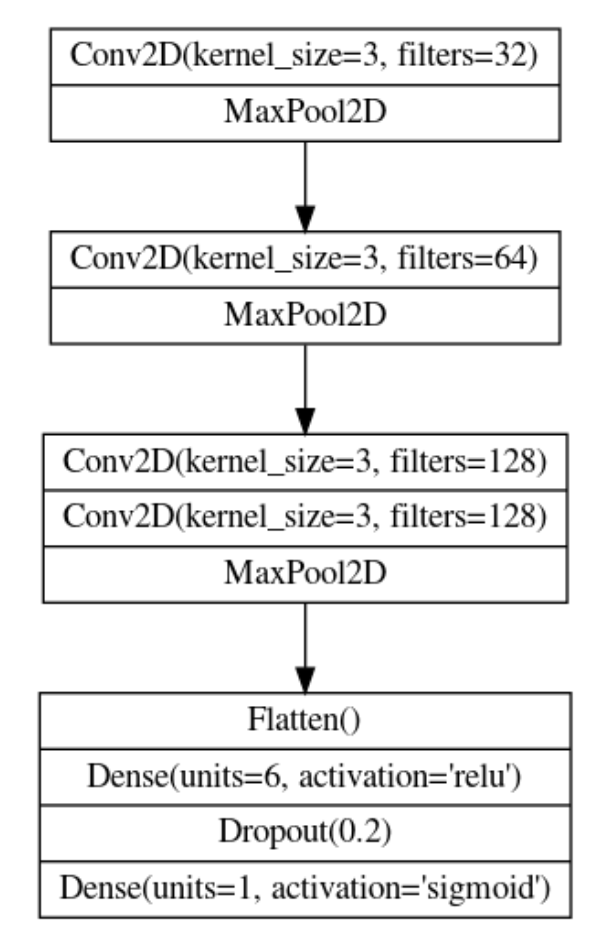
Given the diagram above, complete the model by defining the layers of the third block.

Define Model

from tensorflow import keras
from tensorflow.keras import layers

model = keras.Sequential([
    # Block One
    layers.Conv2D(filters=32, kernel_size=3, activation='relu', padding='same',
                  input_shape=[128, 128, 3]),
    layers.MaxPool2D(),

    # Block Two
    layers.Conv2D(filters=64, kernel_size=3, activation='relu', padding='same'),
    layers.MaxPool2D(),

    # Block Three
    layers.Conv2D(filters=128, kernel_size=3, activation='relu', padding='same'),
    layers.Conv2D(filters=128, kernel_size=3, activation='relu', padding='same'),
    layers.MaxPool2D(),

    # Head
    layers.Flatten(),
    layers.Dense(6, activation='relu'),
    layers.Dropout(0.2),
    layers.Dense(1, activation='sigmoid'),
])

Compile

To prepare for training, compile the model with an appropriate loss and accuracy metric for the “Car or Truck” dataset.

model.compile(
    optimizer=tf.keras.optimizers.Adam(learning_rate=0.0001),
    loss='binary_crossentropy',
    metrics=['binary_accuracy'],
)

Finally, let’s test the performance of this new model. First run this cell to fit the model to the training set.

history = model.fit(
    ds_train,
    validation_data=ds_valid,
    epochs=50,
)

Epoch 1/50
80/80 [==============================] - 36s 348ms/step - loss: 0.6816 - binary_accuracy: 0.5744 - val_loss: 0.6691 - val_binary_accuracy: 0.5785
Epoch 2/50
80/80 [==============================] - 3s 43ms/step - loss: 0.6667 - binary_accuracy: 0.5787 - val_loss: 0.6601 - val_binary_accuracy: 0.5785
Epoch 3/50
80/80 [==============================] - 3s 42ms/step - loss: 0.6613 - binary_accuracy: 0.5787 - val_loss: 0.6503 - val_binary_accuracy: 0.5785
Epoch 4/50
80/80 [==============================] - 3s 42ms/step - loss: 0.6517 - binary_accuracy: 0.5787 - val_loss: 0.6447 - val_binary_accuracy: 0.5785
Epoch 5/50
80/80 [==============================] - 3s 43ms/step - loss: 0.6456 - binary_accuracy: 0.6093 - val_loss: 0.6386 - val_binary_accuracy: 0.5961
Epoch 6/50
80/80 [==============================] - 3s 42ms/step - loss: 0.6372 - binary_accuracy: 0.6330 - val_loss: 0.6354 - val_binary_accuracy: 0.5918
Epoch 7/50
80/80 [==============================] - 4s 44ms/step - loss: 0.6354 - binary_accuracy: 0.6334 - val_loss: 0.6317 - val_binary_accuracy: 0.6129
Epoch 8/50
80/80 [==============================] - 3s 42ms/step - loss: 0.6256 - binary_accuracy: 0.6529 - val_loss: 0.6207 - val_binary_accuracy: 0.6434
Epoch 9/50
80/80 [==============================] - 3s 43ms/step - loss: 0.6205 - binary_accuracy: 0.6635 - val_loss: 0.6137 - val_binary_accuracy: 0.6498
Epoch 10/50
80/80 [==============================] - 3s 42ms/step - loss: 0.6141 - binary_accuracy: 0.6729 - val_loss: 0.6074 - val_binary_accuracy: 0.6680
Epoch 11/50
80/80 [==============================] - 3s 42ms/step - loss: 0.6039 - binary_accuracy: 0.6846 - val_loss: 0.6022 - val_binary_accuracy: 0.6729
Epoch 12/50
80/80 [==============================] - 3s 42ms/step - loss: 0.5969 - binary_accuracy: 0.6998 - val_loss: 0.5973 - val_binary_accuracy: 0.6803
Epoch 13/50
80/80 [==============================] - 3s 42ms/step - loss: 0.5831 - binary_accuracy: 0.7090 - val_loss: 0.5880 - val_binary_accuracy: 0.6967
Epoch 14/50
80/80 [==============================] - 4s 45ms/step - loss: 0.5737 - binary_accuracy: 0.7211 - val_loss: 0.5825 - val_binary_accuracy: 0.7104
Epoch 15/50
80/80 [==============================] - 3s 42ms/step - loss: 0.5616 - binary_accuracy: 0.7299 - val_loss: 0.5712 - val_binary_accuracy: 0.7169
Epoch 16/50
80/80 [==============================] - 3s 43ms/step - loss: 0.5451 - binary_accuracy: 0.7497 - val_loss: 0.5718 - val_binary_accuracy: 0.7090
Epoch 17/50
80/80 [==============================] - 3s 42ms/step - loss: 0.5268 - binary_accuracy: 0.7620 - val_loss: 0.5551 - val_binary_accuracy: 0.7363
Epoch 18/50
80/80 [==============================] - 3s 42ms/step - loss: 0.5020 - binary_accuracy: 0.7880 - val_loss: 0.5333 - val_binary_accuracy: 0.7545
Epoch 19/50
80/80 [==============================] - 3s 42ms/step - loss: 0.4870 - binary_accuracy: 0.7927 - val_loss: 0.5456 - val_binary_accuracy: 0.7355
Epoch 20/50
80/80 [==============================] - 3s 42ms/step - loss: 0.4701 - binary_accuracy: 0.7983 - val_loss: 0.4908 - val_binary_accuracy: 0.7640
Epoch 21/50
80/80 [==============================] - 4s 45ms/step - loss: 0.4308 - binary_accuracy: 0.8085 - val_loss: 0.4861 - val_binary_accuracy: 0.7660
Epoch 22/50
80/80 [==============================] - 3s 42ms/step - loss: 0.3956 - binary_accuracy: 0.8317 - val_loss: 0.4404 - val_binary_accuracy: 0.7989
Epoch 23/50
80/80 [==============================] - 3s 42ms/step - loss: 0.3638 - binary_accuracy: 0.8450 - val_loss: 0.4566 - val_binary_accuracy: 0.7806
Epoch 24/50
80/80 [==============================] - 3s 42ms/step - loss: 0.3382 - binary_accuracy: 0.8607 - val_loss: 0.4534 - val_binary_accuracy: 0.7870
Epoch 25/50
80/80 [==============================] - 3s 42ms/step - loss: 0.3169 - binary_accuracy: 0.8708 - val_loss: 0.4250 - val_binary_accuracy: 0.8127
Epoch 26/50
80/80 [==============================] - 3s 42ms/step - loss: 0.2885 - binary_accuracy: 0.8849 - val_loss: 0.4289 - val_binary_accuracy: 0.8165
Epoch 27/50
80/80 [==============================] - 3s 43ms/step - loss: 0.2668 - binary_accuracy: 0.8904 - val_loss: 0.4419 - val_binary_accuracy: 0.8133
Epoch 28/50
80/80 [==============================] - 3s 42ms/step - loss: 0.2412 - binary_accuracy: 0.9025 - val_loss: 0.4628 - val_binary_accuracy: 0.8070
Epoch 29/50
80/80 [==============================] - 3s 43ms/step - loss: 0.2512 - binary_accuracy: 0.8972 - val_loss: 0.4338 - val_binary_accuracy: 0.7985
Epoch 30/50
80/80 [==============================] - 3s 42ms/step - loss: 0.2250 - binary_accuracy: 0.9150 - val_loss: 0.4218 - val_binary_accuracy: 0.8202
Epoch 31/50
80/80 [==============================] - 3s 42ms/step - loss: 0.2128 - binary_accuracy: 0.9191 - val_loss: 0.4465 - val_binary_accuracy: 0.8377
Epoch 32/50
80/80 [==============================] - 3s 42ms/step - loss: 0.1784 - binary_accuracy: 0.9361 - val_loss: 0.4509 - val_binary_accuracy: 0.8369
Epoch 33/50
80/80 [==============================] - 3s 42ms/step - loss: 0.2013 - binary_accuracy: 0.9234 - val_loss: 0.4551 - val_binary_accuracy: 0.8460
Epoch 34/50
80/80 [==============================] - 3s 42ms/step - loss: 0.1800 - binary_accuracy: 0.9349 - val_loss: 0.4936 - val_binary_accuracy: 0.8414
Epoch 35/50
80/80 [==============================] - 3s 42ms/step - loss: 0.1654 - binary_accuracy: 0.9414 - val_loss: 0.6184 - val_binary_accuracy: 0.8258
Epoch 36/50
80/80 [==============================] - 4s 44ms/step - loss: 0.1439 - binary_accuracy: 0.9478 - val_loss: 0.6884 - val_binary_accuracy: 0.8060
Epoch 37/50
80/80 [==============================] - 3s 42ms/step - loss: 0.1291 - binary_accuracy: 0.9580 - val_loss: 0.7367 - val_binary_accuracy: 0.8155
Epoch 38/50
80/80 [==============================] - 3s 42ms/step - loss: 0.1257 - binary_accuracy: 0.9582 - val_loss: 0.7216 - val_binary_accuracy: 0.8175
Epoch 39/50
80/80 [==============================] - 3s 43ms/step - loss: 0.1313 - binary_accuracy: 0.9541 - val_loss: 0.5901 - val_binary_accuracy: 0.8282
Epoch 40/50
80/80 [==============================] - 3s 42ms/step - loss: 0.1164 - binary_accuracy: 0.9580 - val_loss: 0.7537 - val_binary_accuracy: 0.8167
Epoch 41/50
80/80 [==============================] - 3s 42ms/step - loss: 0.1020 - binary_accuracy: 0.9699 - val_loss: 0.7372 - val_binary_accuracy: 0.8293
Epoch 42/50
80/80 [==============================] - 3s 42ms/step - loss: 0.0985 - binary_accuracy: 0.9687 - val_loss: 0.5475 - val_binary_accuracy: 0.8470
Epoch 43/50
80/80 [==============================] - 3s 42ms/step - loss: 0.1001 - binary_accuracy: 0.9679 - val_loss: 0.6405 - val_binary_accuracy: 0.8386
Epoch 44/50
80/80 [==============================] - 3s 44ms/step - loss: 0.1064 - binary_accuracy: 0.9613 - val_loss: 0.5989 - val_binary_accuracy: 0.8284
Epoch 45/50
80/80 [==============================] - 3s 42ms/step - loss: 0.0996 - binary_accuracy: 0.9695 - val_loss: 0.5213 - val_binary_accuracy: 0.8311
Epoch 46/50
80/80 [==============================] - 3s 42ms/step - loss: 0.0823 - binary_accuracy: 0.9740 - val_loss: 0.6159 - val_binary_accuracy: 0.8052
Epoch 47/50
80/80 [==============================] - 3s 43ms/step - loss: 0.0737 - binary_accuracy: 0.9773 - val_loss: 0.6454 - val_binary_accuracy: 0.8359
Epoch 48/50
80/80 [==============================] - 3s 42ms/step - loss: 0.0721 - binary_accuracy: 0.9791 - val_loss: 0.6538 - val_binary_accuracy: 0.8491
Epoch 49/50
80/80 [==============================] - 3s 43ms/step - loss: 0.0684 - binary_accuracy: 0.9797 - val_loss: 0.6213 - val_binary_accuracy: 0.8418
Epoch 50/50
80/80 [==============================] - 3s 42ms/step - loss: 0.0623 - binary_accuracy: 0.9803 - val_loss: 0.7014 - val_binary_accuracy: 0.8517

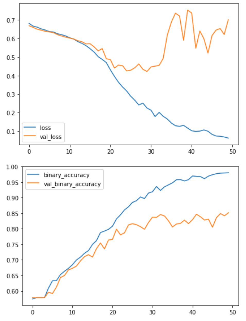
Train the Model

How would you interpret these training curves? Did this model improve upon the model from the tutorial?

The learning curves for the model from the tutorial diverged fairly rapidly. This would indicate that it was prone to overfitting and in need of some regularization. The additional layer in our new model would make it even more prone to overfitting. However, adding some regularization with the Dropout layer helped prevent this. These changes improved the validation accuracy of the model by several points.

These exercises showed you how to design a custom convolutional network to solve a specific classification problem. Though most models these days will be built on top of a pretrained base, it certain circumstances a smaller custom convnet might still be preferable – such as with a smaller or unusual dataset or when computing resources are very limited. As you saw here, for certain problems they can perform just as well as a pretrained model.