Data Augmentation

Now that you’ve learned the fundamentals of convolutional classifiers, you’re ready to move on to more advanced topics.

In this lesson, you’ll learn a trick that can give a boost to your image classifiers: it’s called data augmentation.

The Usefulness of Fake Data

The best way to improve the performance of a machine learning model is to train it on more data. The more examples the model has to learn from, the better it will be able to recognize which differences in images matter and which do not. More data helps the model to generalize better.

One easy way of getting more data is to use the data you already have. If we can transform the images in our dataset in ways that preserve the class, we can teach our classifier to ignore those kinds of transformations. For instance, whether a car is facing left or right in a photo doesn’t change the fact that it is a Car and not a Truck. So, if we augment our training data with flipped images, our classifier will learn that “left or right” is a difference it should ignore.

And that’s the whole idea behind data augmentation: add in some extra fake data that looks reasonably like the real data and your classifier will improve.

Using Data Augmentation

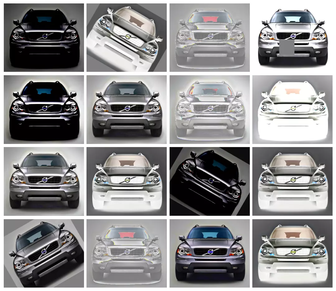
Typically, many kinds of transformation are used when augmenting a dataset. These might include rotating the image, adjusting the color or contrast, warping the image, or many other things, usually applied in combination. Here is a sample of the different ways a single image might be transformed.

Data augmentation is usually done online, meaning, as the images are being fed into the network for training. Recall that training is usually done on mini-batches of data. This is what a batch of 16 images might look like when data augmentation is used.

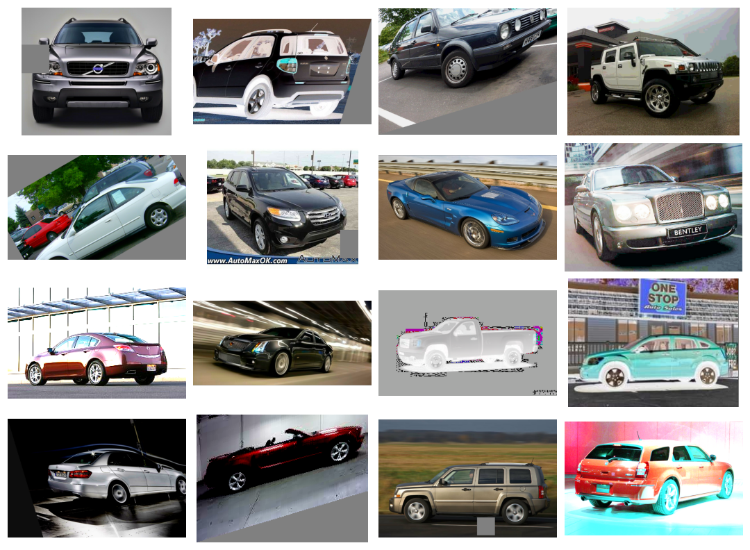
Each time an image is used during training, a new random transformation is applied. This way, the model is always seeing something a little different than what it’s seen before. This extra variance in the training data is what helps the model on new data.

It’s important to remember though that not every transformation will be useful on a given problem. Most importantly, whatever transformations you use should not mix up the classes. If you were training a digit recognizer, for instance, rotating images would mix up ‘9’s and ‘6’s. In the end, the best approach for finding good augmentations is the same as with most ML problems: try it and see!

Example - Training with Data Augmentation

Keras lets you augment your data in two ways. The first way is to include it in the data pipeline with a function like ImageDataGenerator. The second way is to include it in the model definition by using Keras’s preprocessing layers. This is the approach that we’ll take. The primary advantage for us is that the image transformations will be computed on the GPU instead of the CPU, potentially speeding up training.

# Imports
import os, warnings
import matplotlib.pyplot as plt
from matplotlib import gridspec

import numpy as np
import tensorflow as tf
from tensorflow.keras.preprocessing import image_dataset_from_directory

# Reproducability
def set_seed(seed=31415):
    np.random.seed(seed)
    tf.random.set_seed(seed)
    os.environ['PYTHONHASHSEED'] = str(seed)
    os.environ['TF_DETERMINISTIC_OPS'] = '1'
set_seed()

# Set Matplotlib defaults
plt.rc('figure', autolayout=True)
plt.rc('axes', labelweight='bold', labelsize='large',
       titleweight='bold', titlesize=18, titlepad=10)
plt.rc('image', cmap='magma')
warnings.filterwarnings("ignore") # to clean up output cells


# Load training and validation sets
ds_train_ = image_dataset_from_directory(
    '../input/car-or-truck/train',
    labels='inferred',
    label_mode='binary',
    image_size=[128, 128],
    interpolation='nearest',
    batch_size=64,
    shuffle=True,
)
ds_valid_ = image_dataset_from_directory(
    '../input/car-or-truck/valid',
    labels='inferred',
    label_mode='binary',
    image_size=[128, 128],
    interpolation='nearest',
    batch_size=64,
    shuffle=False,
)

# Data Pipeline
def convert_to_float(image, label):
    image = tf.image.convert_image_dtype(image, dtype=tf.float32)
    return image, label

AUTOTUNE = tf.data.experimental.AUTOTUNE
ds_train = (
    ds_train_
    .map(convert_to_float)
    .cache()
    .prefetch(buffer_size=AUTOTUNE)
)
ds_valid = (
    ds_valid_
    .map(convert_to_float)
    .cache()
    .prefetch(buffer_size=AUTOTUNE)
)

Define Model

To illustrate the effect of augmentation, we’ll just add a couple of simple transformations to the model from Tutorial 1.

from tensorflow import keras
from tensorflow.keras import layers
# these are a new feature in TF 2.2
from tensorflow.keras.layers.experimental import preprocessing


pretrained_base = tf.keras.models.load_model(
    '../input/cv-course-models/cv-course-models/vgg16-pretrained-base',
)
pretrained_base.trainable = False

model = keras.Sequential([
    # Preprocessing
    preprocessing.RandomFlip('horizontal'), # flip left-to-right
    preprocessing.RandomContrast(0.5), # contrast change by up to 50%
    # Base
    pretrained_base,
    # Head
    layers.Flatten(),
    layers.Dense(6, activation='relu'),
    layers.Dense(1, activation='sigmoid'),
])

Train and Evaluate

model.compile(
    optimizer='adam',
    loss='binary_crossentropy',
    metrics=['binary_accuracy'],
)

history = model.fit(
    ds_train,
    validation_data=ds_valid,
    epochs=30,
    verbose=0,
)

import pandas as pd

history_frame = pd.DataFrame(history.history)

history_frame.loc[:, ['loss', 'val_loss']].plot()
history_frame.loc[:, ['binary_accuracy', 'val_binary_accuracy']].plot();

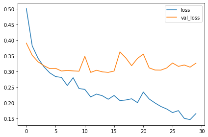
The training and validation curves in the model from Tutorial 1 diverged fairly quickly, suggesting that it could benefit from some regularization. The learning curves for this model were able to stay closer together, and we achieved some modest improvement in validation loss and accuracy. This suggests that the dataset did indeed benefit from the augmentation.

Exercises

In these exercises, you’ll explore what effect various random transformations have on an image, consider what kind of augmentation might be appropriate on a given dataset, and then use data augmentation with the Car or Truck dataset to train a custom network.

from tensorflow import keras
from tensorflow.keras import layers
from tensorflow.keras.layers.experimental import preprocessing

# Imports
import os, warnings
import matplotlib.pyplot as plt
from matplotlib import gridspec

import numpy as np
import tensorflow as tf
from tensorflow.keras.preprocessing import image_dataset_from_directory

# Reproducability
def set_seed(seed=31415):
    np.random.seed(seed)
    tf.random.set_seed(seed)
    os.environ['PYTHONHASHSEED'] = str(seed)
    os.environ['TF_DETERMINISTIC_OPS'] = '1'
set_seed()

# Set Matplotlib defaults
plt.rc('figure', autolayout=True)
plt.rc('axes', labelweight='bold', labelsize='large',
       titleweight='bold', titlesize=18, titlepad=10)
plt.rc('image', cmap='magma')
warnings.filterwarnings("ignore") # to clean up output cells


# Load training and validation sets
ds_train_ = image_dataset_from_directory(
    '../input/car-or-truck/train',
    labels='inferred',
    label_mode='binary',
    image_size=[128, 128],
    interpolation='nearest',
    batch_size=64,
    shuffle=True,
)
ds_valid_ = image_dataset_from_directory(
    '../input/car-or-truck/valid',
    labels='inferred',
    label_mode='binary',
    image_size=[128, 128],
    interpolation='nearest',
    batch_size=64,
    shuffle=False,
)

# Data Pipeline
def convert_to_float(image, label):
    image = tf.image.convert_image_dtype(image, dtype=tf.float32)
    return image, label

AUTOTUNE = tf.data.experimental.AUTOTUNE
ds_train = (
    ds_train_
    .map(convert_to_float)
    .cache()
    .prefetch(buffer_size=AUTOTUNE)
)
ds_valid = (
    ds_valid_
    .map(convert_to_float)
    .cache()
    .prefetch(buffer_size=AUTOTUNE)
)

Explore Augmentation

Uncomment a transformation and run the cell to see what it does. You can experiment with the parameter values too, if you like. (The factor parameters should be greater than 0 and, generally, less than 1.) Run the cell again if you’d like to get a new random image.

# all of the "factor" parameters indicate a percent-change
augment = keras.Sequential([
    # preprocessing.RandomContrast(factor=0.5),
    preprocessing.RandomFlip(mode='horizontal'), # meaning, left-to-right
    # preprocessing.RandomFlip(mode='vertical'), # meaning, top-to-bottom
    # preprocessing.RandomWidth(factor=0.15), # horizontal stretch
    # preprocessing.RandomRotation(factor=0.20),
    # preprocessing.RandomTranslation(height_factor=0.1, width_factor=0.1),
])


ex = next(iter(ds_train.unbatch().map(lambda x, y: x).batch(1)))

plt.figure(figsize=(10,10))
for i in range(16):
    image = augment(ex, training=True)
    plt.subplot(4, 4, i+1)
    plt.imshow(tf.squeeze(image))
    plt.axis('off')
plt.show()

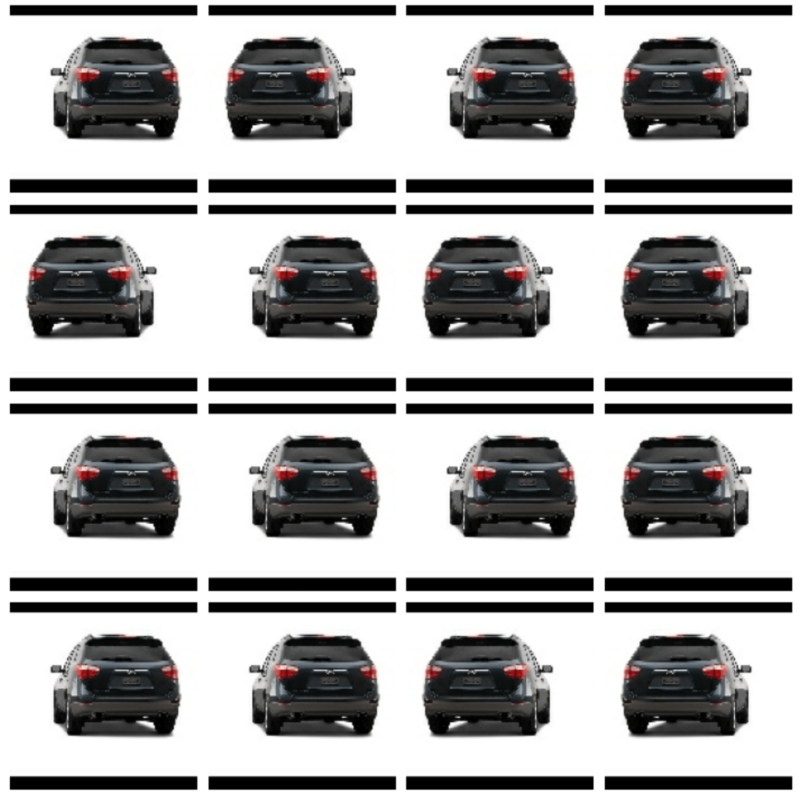
Do the transformations you chose seem reasonable for the Car or Truck dataset?

In this exercise, we’ll look at a few datasets and think about what kind of augmentation might be appropriate. Your reasoning might be different that what we discuss in the solution. That’s okay. The point of these problems is just to think about how a transformation might interact with a classification problem – for better or worse.

The EuroSAT dataset consists of satellite images of the Earth classified by geographic feature. Below are a number of images from this dataset.

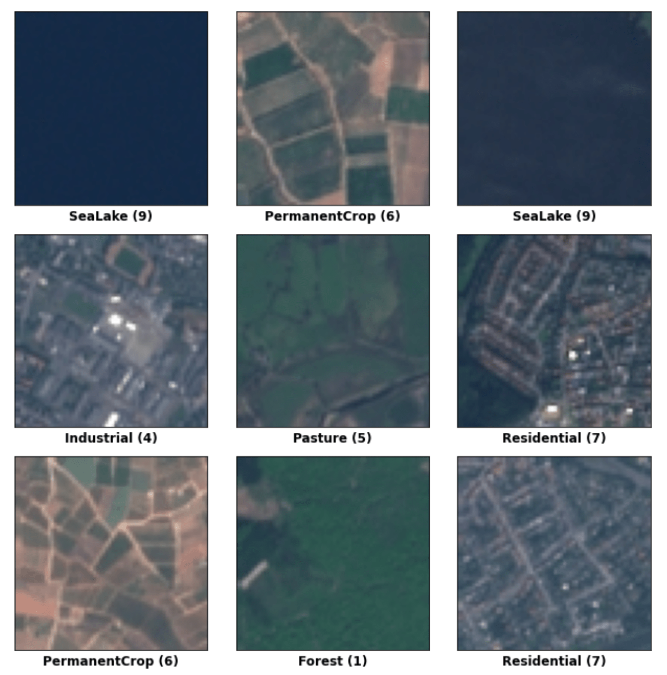
EuroSAT

What kinds of transformations might be appropriate for this dataset?

It seems to this author that flips and rotations would be worth trying first since there’s no concept of orientation for pictures taken straight overhead. None of the transformations seem likely to confuse classes, however.

The TensorFlow Flowers dataset consists of photographs of flowers of several species. Below is a sample.

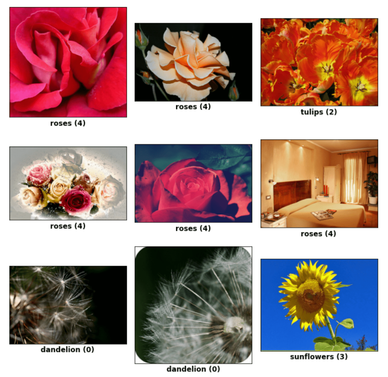
TensorFlow Flowers

What kinds of transformations might be appropriate for the TensorFlow Flowers dataset?

It seems to this author that horizontal flips and moderate rotations would be worth trying first. Some augmentation libraries include transformations of hue (like red to blue). Since the color of a flower seems distinctive of its class, a change of hue might be less successful. On the other hand, there is suprising variety in cultivated flowers like roses, so, depending on the dataset, this might be an improvement after all!

Now you’ll use data augmentation with a custom convnet similar to the one you built in Exercise 5. Since data augmentation effectively increases the size of the dataset, we can increase the capacity of the model in turn without as much risk of overfitting.

Add Preprocessing Layers

from tensorflow import keras
from tensorflow.keras import layers

model = keras.Sequential([
    layers.InputLayer(input_shape=[128, 128, 3]),

    # Data Augmentation
    preprocessing.RandomContrast(factor=0.10),
    preprocessing.RandomFlip(mode='horizontal'),
    preprocessing.RandomRotation(factor=0.10),

    # Block One
    layers.BatchNormalization(renorm=True),
    layers.Conv2D(filters=64, kernel_size=3, activation='relu', padding='same'),
    layers.MaxPool2D(),

    # Block Two
    layers.BatchNormalization(renorm=True),
    layers.Conv2D(filters=128, kernel_size=3, activation='relu', padding='same'),
    layers.MaxPool2D(),

    # Block Three
    layers.BatchNormalization(renorm=True),
    layers.Conv2D(filters=256, kernel_size=3, activation='relu', padding='same'),
    layers.Conv2D(filters=256, kernel_size=3, activation='relu', padding='same'),
    layers.MaxPool2D(),

    # Head
    layers.BatchNormalization(renorm=True),
    layers.Flatten(),
    layers.Dense(8, activation='relu'),
    layers.Dense(1, activation='sigmoid'),
])

Now we’ll train the model. Run the next cell to compile it with a loss and accuracy metric and fit it to the training set.

optimizer = tf.keras.optimizers.Adam(epsilon=0.01)
model.compile(
    optimizer=optimizer,
    loss='binary_crossentropy',
    metrics=['binary_accuracy'],
)

history = model.fit(
    ds_train,
    validation_data=ds_valid,
    epochs=50,
)

# Plot learning curves
import pandas as pd
history_frame = pd.DataFrame(history.history)
history_frame.loc[:, ['loss', 'val_loss']].plot()
history_frame.loc[:, ['binary_accuracy', 'val_binary_accuracy']].plot();

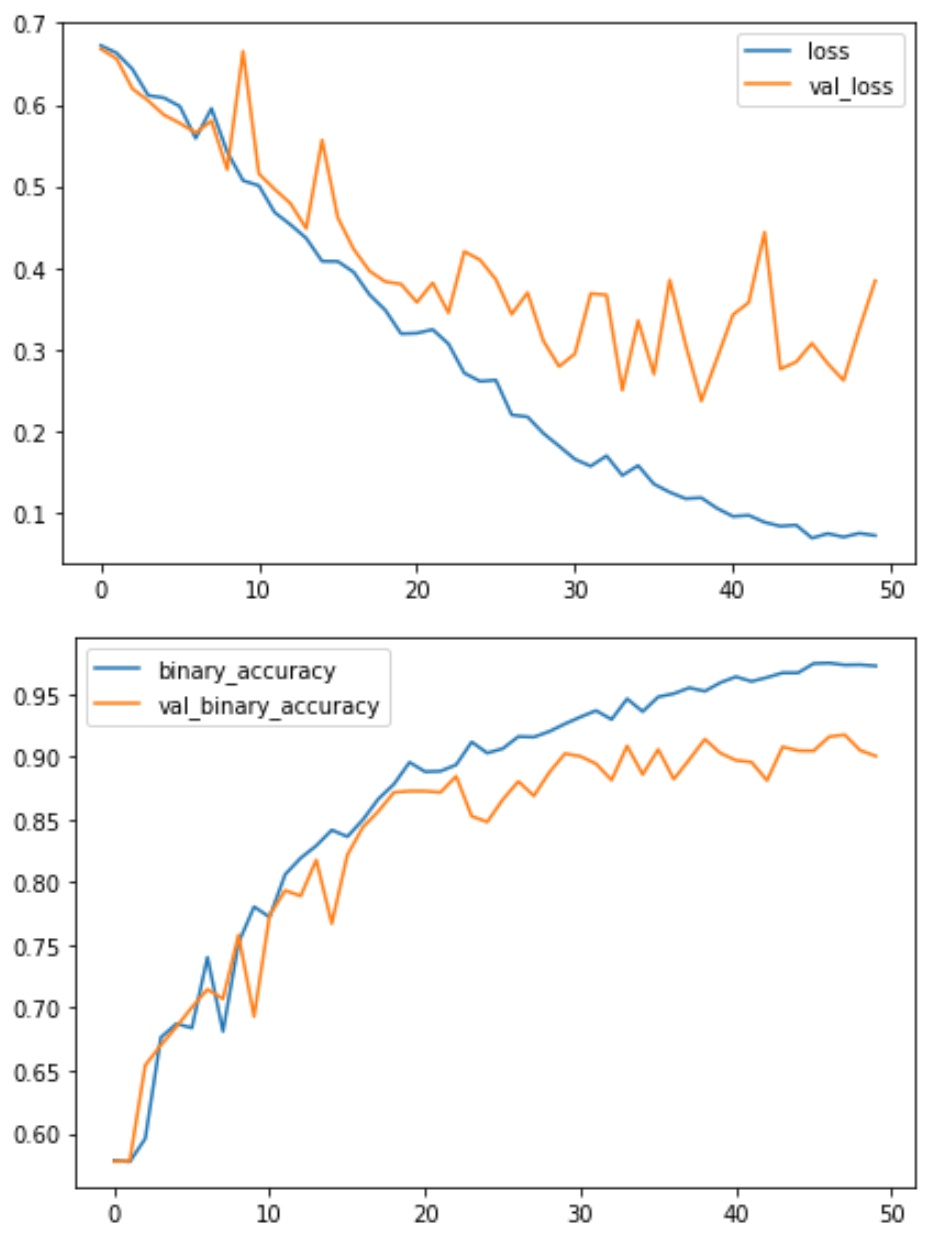
Train Model

Examine the training curves. Was there any sign of overfitting? How does the performance of this model compare to other models you’ve trained in this course?

Data augmentation is a powerful and commonly-used tool to improve model training, not only for convolutional networks, but for many other kinds of neural network models as well. Whatever your problem, the principle remains the same: you can make up for an inadequacy in your data by adding in “fake” data to cover it over. Experimenting with augmentations is a great way to find out just how far your data can go!