Interactive Maps

Your first interactive map

We begin by creating a relatively simple map with folium.Map().

import pandas as pd
import geopandas as gpd
import math
import folium
from folium import Choropleth, Circle, Marker
from folium.plugins import HeatMap, MarkerCluster

def embed_map(m, file_name):
    from IPython.display import IFrame
    m.save(file_name)
    return IFrame(file_name, width='100%', height='500px')

# Create a map
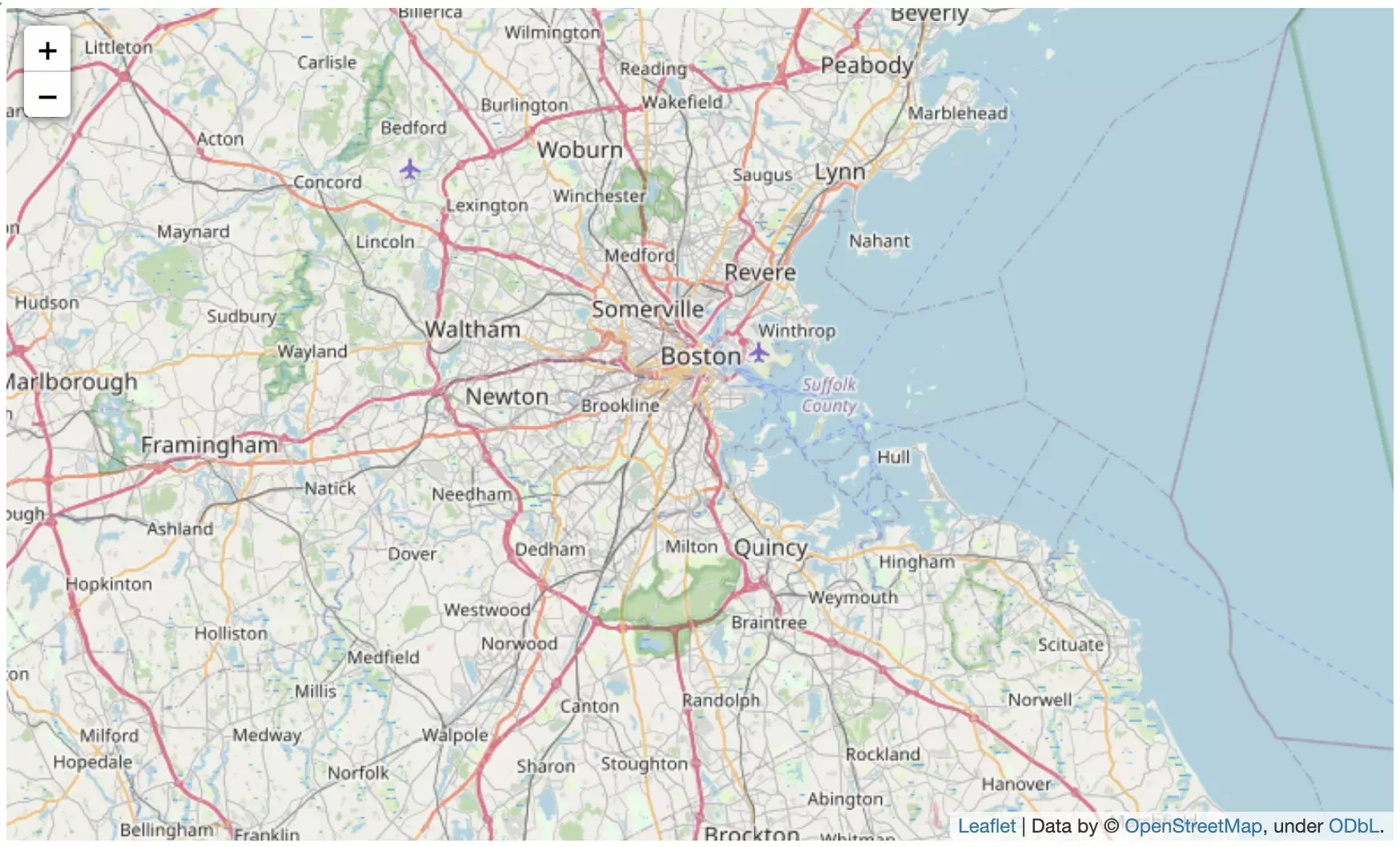
m_1 = folium.Map(location=[42.32,-71.0589], tiles='openstreetmap', zoom_start=10)

# Display the map
embed_map(m_1, "q_1.html")

Several arguments customize the appearance of the map:

• location sets the initial center of the map. We use the latitude (42.32° N) and longitude (-71.0589° E) of the city of Boston.
• tiles changes the styling of the map; in this case, we choose the OpenStreetMap style. If you’re curious, you can find the other options listed here.
• zoom_start sets the initial level of zoom of the map, where higher values zoom in closer to the map. Take the time now to explore by zooming in and out, or by dragging the map in different directions.

The data

Now, we’ll add some crime data to the map!

We won’t focus on the data loading step. Instead, you can imagine you are at a point where you already have the data in a pandas DataFrame crimes. The first five rows of the data are shown below.

# Load the data
crimes = pd.read_csv("crime.csv", encoding='latin-1')

# Drop rows with missing locations
crimes.dropna(subset=['Lat', 'Long', 'DISTRICT'], inplace=True)

# Focus on major crimes in 2018
crimes = crimes[crimes.OFFENSE_CODE_GROUP.isin([
    'Larceny', 'Auto Theft', 'Robbery', 'Larceny From Motor Vehicle', 'Residential Burglary',
    'Simple Assault', 'Harassment', 'Ballistics', 'Aggravated Assault', 'Other Burglary', 
    'Arson', 'Commercial Burglary', 'HOME INVASION', 'Homicide', 'Criminal Harassment', 
    'Manslaughter'])]
crimes = crimes[crimes.YEAR>=2018]

# Print the first five rows of the table
crimes.head()

	INCIDENT_NUMBER	OFFENSE_CODE	OFFENSE_CODE_GROUP	OFFENSE_DESCRIPTION	DISTRICT	REPORTING_AREA	SHOOTING	OCCURRED_ON_DATE	YEAR	MONTH	DAY_OF_WEEK	HOUR	UCR_PART	STREET	Lat	Long	Location
0	I182070945	619	Larceny	LARCENY ALL OTHERS	D14	808	NaN	2018-09-02 13:00:00	2018	9	Sunday	13	Part One	LINCOLN ST	42.357791	-71.139371	(42.35779134, -71.13937053)
6	I182070933	724	Auto Theft	AUTO THEFT	B2	330	NaN	2018-09-03 21:25:00	2018	9	Monday	21	Part One	NORMANDY ST	42.306072	-71.082733	(42.30607218, -71.08273260)
8	I182070931	301	Robbery	ROBBERY - STREET	C6	177	NaN	2018-09-03 20:48:00	2018	9	Monday	20	Part One	MASSACHUSETTS AVE	42.331521	-71.070853	(42.33152148, -71.07085307)
19	I182070915	614	Larceny From Motor Vehicle	LARCENY THEFT FROM MV - NON-ACCESSORY	B2	181	NaN	2018-09-02 18:00:00	2018	9	Sunday	18	Part One	SHIRLEY ST	42.325695	-71.068168	(42.32569490, -71.06816778)
24	I182070908	522	Residential Burglary	BURGLARY - RESIDENTIAL - NO FORCE	B2	911	NaN	2018-09-03 18:38:00	2018	9	Monday	18	Part One	ANNUNCIATION RD	42.335062	-71.093168	(42.33506218, -71.09316781)

Plotting points

To reduce the amount of data we need to fit on the map, we’ll (temporarily) confine our attention to daytime robberies.

daytime_robberies = crimes[((crimes.OFFENSE_CODE_GROUP == 'Robbery') & \
                            (crimes.HOUR.isin(range(9,18))))]

folium.Marker

We add markers to the map with folium.Marker(). Each marker below corresponds to a different robbery.

# Create a map
m_2 = folium.Map(location=[42.32,-71.0589], tiles='cartodbpositron', zoom_start=13)

# Add points to the map
for idx, row in daytime_robberies.iterrows():
    Marker([row['Lat'], row['Long']]).add_to(m_2)

# Display the map
embed_map(m_2, "q_2.html")

folium.plugins.MarkerCluster

If we have a lot of markers to add, folium.plugins.MarkerCluster() can help to declutter the map. Each marker is added to a MarkerCluster object.

# Create the map
m_3 = folium.Map(location=[42.32,-71.0589], tiles='cartodbpositron', zoom_start=13)

# Add points to the map
mc = MarkerCluster()
for idx, row in daytime_robberies.iterrows():
    if not math.isnan(row['Long']) and not math.isnan(row['Lat']):
        mc.add_child(Marker([row['Lat'], row['Long']]))
m_3.add_child(mc)

# Display the map
embed_map(m_3, "q_3.html")

Bubble maps

A bubble map uses circles instead of markers. By varying the size and color of each circle, we can also show the relationship between location and two other variables.

We create a bubble map by using folium.Circle() to iteratively add circles. In the code cell below, robberies that occurred in hours 9-12 are plotted in green, whereas robberies from hours 13-17 are plotted in red.

# Create a base map
m_4 = folium.Map(location=[42.32,-71.0589], tiles='cartodbpositron', zoom_start=13)

def color_producer(val):
    if val <= 12:
        return 'forestgreen'
    else:
        return 'darkred'

# Add a bubble map to the base map
for i in range(0,len(daytime_robberies)):
    Circle(
        location=[daytime_robberies.iloc[i]['Lat'], daytime_robberies.iloc[i]['Long']],
        radius=20,
        color=color_producer(daytime_robberies.iloc[i]['HOUR'])).add_to(m_4)

# Display the map
embed_map(m_4, "q_4.html")

Note that folium.Circle() takes several arguments:

• location is a list containing the center of the circle, in latitude and longitude.
• radius sets the radius of the circle.
  • Note that in a traditional bubble map, the radius of each circle is allowed to vary. We can implement this by defining a function similar to the color_producer() function that is used to vary the color of each circle.
• color sets the color of each circle.
  • The color_producer() function is used to visualize the effect of the hour on robbery location.

Heatmaps

To create a heatmap, we use folium.plugins.HeatMap(). This shows the density of crime in different areas of the city, where red areas have relatively more criminal incidents.

As we’d expect for a big city, most of the crime happens near the center.

# Create a base map
m_5 = folium.Map(location=[42.32,-71.0589], tiles='cartodbpositron', zoom_start=12)

# Add a heatmap to the base map
HeatMap(data=crimes[['Lat', 'Long']], radius=10).add_to(m_5)

# Display the map
embed_map(m_5, "q_5.html")