Overfitting and Underfitting
Recall from the example in the previous lesson that Keras will keep a history of the training and validation loss over the epochs that it is training the model. In this lesson, we’re going to learn how to interpret these learning curves and how we can use them to guide model development. In particular, we’ll examine at the learning curves for evidence of underfitting and overfitting and look at a couple of strategies for correcting it.
Interpreting the Learning Curves
You might think about the information in the training data as being of two kinds: signal and noise. The signal is the part that generalizes, the part that can help our model make predictions from new data. The noise is that part that is only true of the training data; the noise is all of the random fluctuation that comes from data in the real-world or all of the incidental, non-informative patterns that can’t actually help the model make predictions. The noise is the part might look useful but really isn’t.
We train a model by choosing weights or parameters that minimize the loss on a training set. You might know, however, that to accurately assess a model’s performance, we need to evaluate it on a new set of data, the validation data.
When we train a model we’ve been plotting the loss on the training set epoch by epoch. To this we’ll add a plot the validation data too. These plots we call the learning curves. To train deep learning models effectively, we need to be able to interpret them.
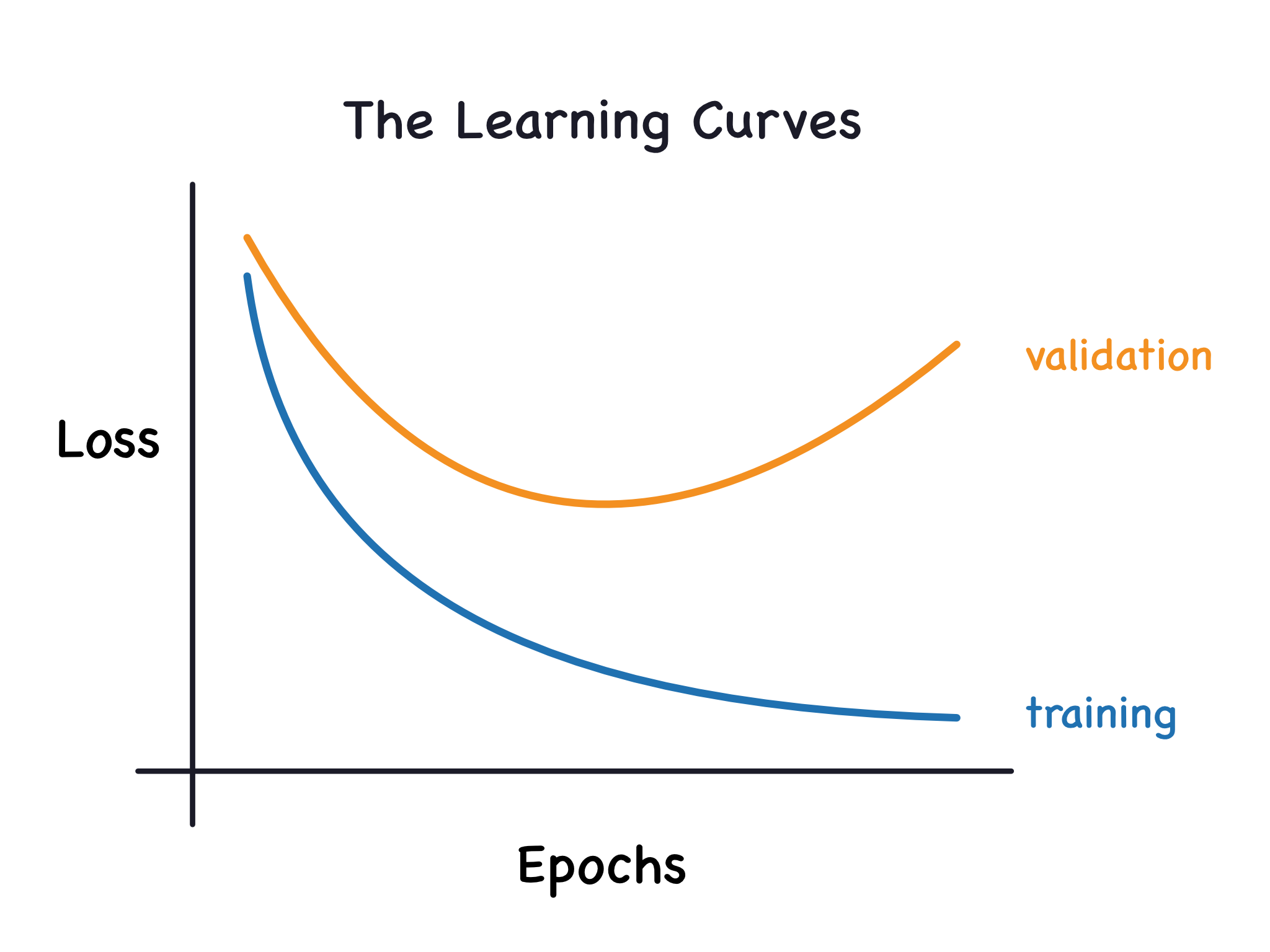
Now, the training loss will go down either when the model learns signal or when it learns noise. But the validation loss will go down only when the model learns signal. (Whatever noise the model learned from the training set won’t generalize to new data.) So, when a model learns signal both curves go down, but when it learns noise a gap is created in the curves. The size of the gap tells you how much noise the model has learned.
Ideally, we would create models that learn all of the signal and none of the noise. This will practically never happen. Instead we make a trade. We can get the model to learn more signal at the cost of learning more noise. So long as the trade is in our favor, the validation loss will continue to decrease. After a certain point, however, the trade can turn against us, the cost exceeds the benefit, and the validation loss begins to rise.
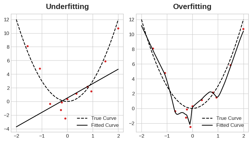
This trade-off indicates that there can be two problems that occur when training a model: not enough signal or too much noise. Underfitting the training set is when the loss is not as low as it could be because the model hasn’t learned enough signal. Overfitting the training set is when the loss is not as low as it could be because the model learned too much noise. The trick to training deep learning models is finding the best balance between the two.
We’ll look at a couple ways of getting more signal out of the training data while reducing the amount of noise.
Capacity
A model’s capacity refers to the size and complexity of the patterns it is able to learn. For neural networks, this will largely be determined by how many neurons it has and how they are connected together. If it appears that your network is underfitting the data, you should try increasing its capacity.
You can increase the capacity of a network either by making it wider (more units to existing layers) or by making it deeper (adding more layers). Wider networks have an easier time learning more linear relationships, while deeper networks prefer more nonlinear ones. Which is better just depends on the dataset.
model = keras.Sequential([
    layers.Dense(16, activation='relu'),
    layers.Dense(1),
])

wider = keras.Sequential([
    layers.Dense(32, activation='relu'),
    layers.Dense(1),
])

deeper = keras.Sequential([
    layers.Dense(16, activation='relu'),
    layers.Dense(16, activation='relu'),
    layers.Dense(1),
])
The capacity of a network can affect its performance.
Early Stopping
We mentioned that when a model is too eagerly learning noise, the validation loss may start to increase during training. To prevent this, we can simply stop the training whenever it seems the validation loss isn’t decreasing anymore. Interrupting the training this way is called early stopping.
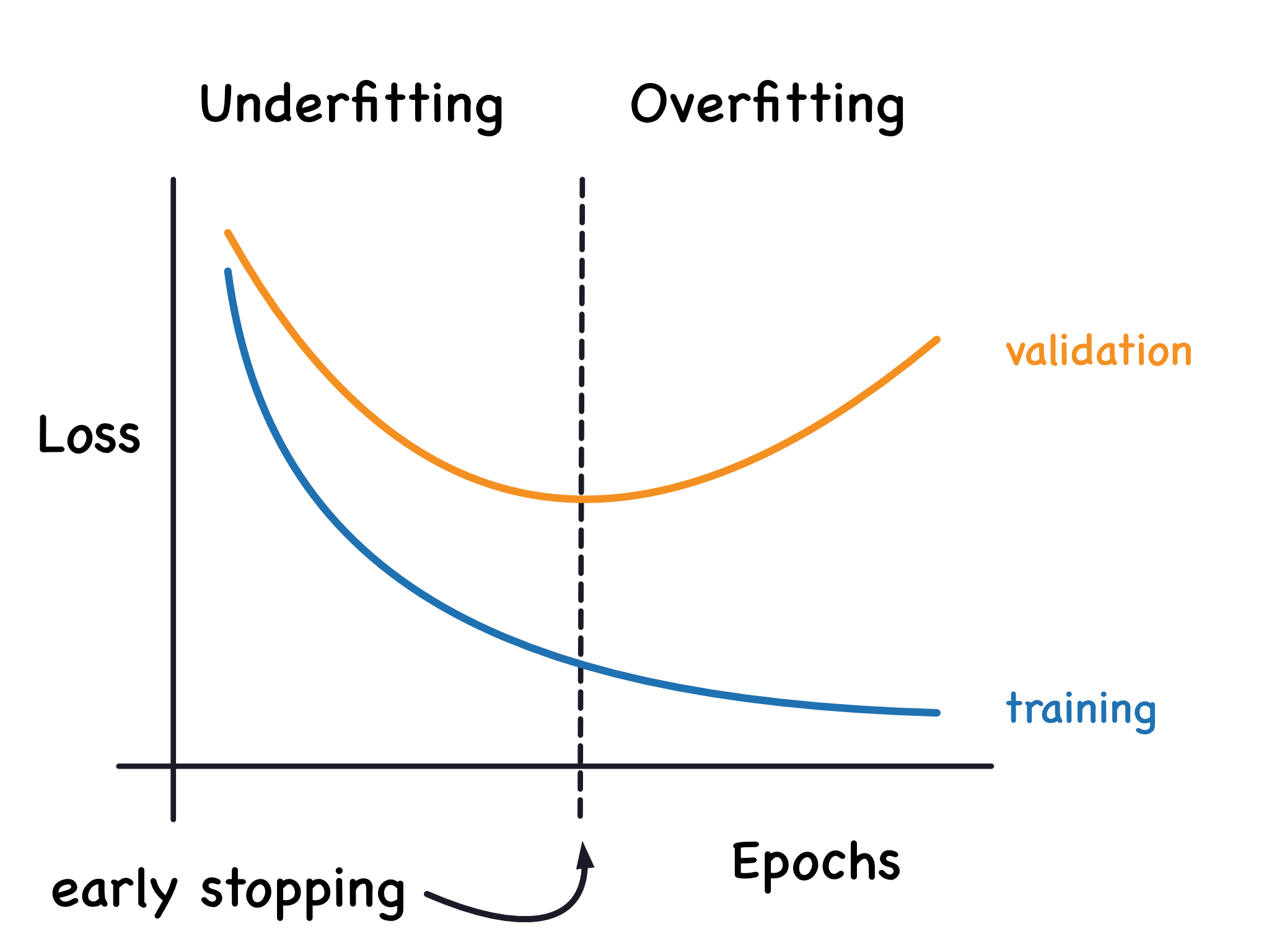
Once we detect that the validation loss is starting to rise again, we can reset the weights back to where the minimum occured. This ensures that the model won’t continue to learn noise and overfit the data.
Training with early stopping also means we’re in less danger of stopping the training too early, before the network has finished learning signal. So besides preventing overfitting from training too long, early stopping can also prevent underfitting from not training long enough. Just set your training epochs to some large number (more than you’ll need), and early stopping will take care of the rest.
Adding Early Stopping
In Keras, we include early stopping in our training through a callback. A callback is just a function you want run every so often while the network trains. The early stopping callback will run after every epoch. (Keras has a variety of useful callbacks pre-defined, but you can define your own, too.)
from tensorflow.keras.callbacks import EarlyStopping

early_stopping = EarlyStopping(
    min_delta=0.001, # minimium amount of change to count as an improvement
    patience=20, # how many epochs to wait before stopping
    restore_best_weights=True,
)
These parameters say: “If there hasn’t been at least an improvement of 0.001 in the validation loss over the previous 20 epochs, then stop the training and keep the best model you found.” It can sometimes be hard to tell if the validation loss is rising due to overfitting or just due to random batch variation. The parameters allow us to set some allowances around when to stop.
As we’ll see in our example, we’ll pass this callback to the fit method along with the loss and optimizer.
Example - Train a Model with Early Stopping
Let’s continue developing the model from the example in the last tutorial. We’ll increase the capacity of that network but also add an early-stopping callback to prevent overfitting.
Here’s the data prep again.
import pandas as pd
from IPython.display import display

red_wine = pd.read_csv('../input/dl-course-data/red-wine.csv')

# Create training and validation splits
df_train = red_wine.sample(frac=0.7, random_state=0)
df_valid = red_wine.drop(df_train.index)
display(df_train.head(4))

# Scale to [0, 1]
max_ = df_train.max(axis=0)
min_ = df_train.min(axis=0)
df_train = (df_train - min_) / (max_ - min_)
df_valid = (df_valid - min_) / (max_ - min_)

# Split features and target
X_train = df_train.drop('quality', axis=1)
X_valid = df_valid.drop('quality', axis=1)
y_train = df_train['quality']
y_valid = df_valid['quality']
| fixed acidity | volatile acidity | citric acid | residual sugar | chlorides | free sulfur dioxide | total sulfur dioxide | density | pH | sulphates | alcohol | quality | |
|---|---|---|---|---|---|---|---|---|---|---|---|---|
| 1109 | 10.8 | 0.470 | 0.43 | 2.10 | 0.171 | 27.0 | 66.0 | 0.99820 | 3.17 | 0.76 | 10.8 | 6 |
| 1032 | 8.1 | 0.820 | 0.00 | 4.10 | 0.095 | 5.0 | 14.0 | 0.99854 | 3.36 | 0.53 | 9.6 | 5 |
| 1002 | 9.1 | 0.290 | 0.33 | 2.05 | 0.063 | 13.0 | 27.0 | 0.99516 | 3.26 | 0.84 | 11.7 | 7 |
| 487 | 10.2 | 0.645 | 0.36 | 1.80 | 0.053 | 5.0 | 14.0 | 0.99820 | 3.17 | 0.42 | 10.0 | 6 |
Now let’s increase the capacity of the network. We’ll go for a fairly large network, but rely on the callback to halt the training once the validation loss shows signs of increasing.
from tensorflow import keras
from tensorflow.keras import layers, callbacks

early_stopping = callbacks.EarlyStopping(
    min_delta=0.001, # minimium amount of change to count as an improvement
    patience=20, # how many epochs to wait before stopping
    restore_best_weights=True,
)

model = keras.Sequential([
    layers.Dense(512, activation='relu', input_shape=[11]),
    layers.Dense(512, activation='relu'),
    layers.Dense(512, activation='relu'),
    layers.Dense(1),
])
model.compile(
    optimizer='adam',
    loss='mae',
)
After defining the callback, add it as an argument in fit (you can have several, so put it in a list). Choose a large number of epochs when using early stopping, more than you’ll need.
history = model.fit(
    X_train, y_train,
    validation_data=(X_valid, y_valid),
    batch_size=256,
    epochs=500,
    callbacks=[early_stopping], # put your callbacks in a list
    verbose=0,  # turn off training log
)

history_df = pd.DataFrame(history.history)
history_df.loc[:, ['loss', 'val_loss']].plot();
print("Minimum validation loss: {}".format(history_df['val_loss'].min()))
2021-11-09 00:10:50.873509: I tensorflow/compiler/mlir/mlir_graph_optimization_pass.cc:185] None of the MLIR Optimization Passes are enabled (registered 2)
Minimum validation loss: 0.09031068533658981
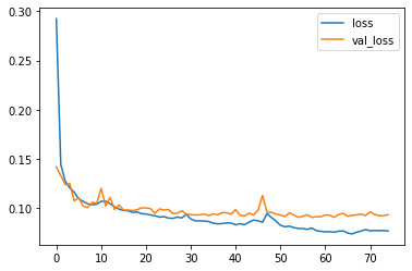
And sure enough, Keras stopped the training well before the full 500 epochs!
Spotify Example
# Setup plotting
import matplotlib.pyplot as plt
plt.style.use('seaborn-whitegrid')
# Set Matplotlib defaults
plt.rc('figure', autolayout=True)
plt.rc('axes', labelweight='bold', labelsize='large',
       titleweight='bold', titlesize=18, titlepad=10)
plt.rc('animation', html='html5')
First load the Spotify dataset. Your task will be to predict the popularity of a song based on various audio features, like ‘tempo’, ‘danceability’, and ‘mode’.
import pandas as pd
from sklearn.preprocessing import StandardScaler, OneHotEncoder
from sklearn.compose import make_column_transformer
from sklearn.model_selection import GroupShuffleSplit

from tensorflow import keras
from tensorflow.keras import layers
from tensorflow.keras import callbacks

spotify = pd.read_csv('../input/dl-course-data/spotify.csv')

X = spotify.copy().dropna()
y = X.pop('track_popularity')
artists = X['track_artist']

features_num = ['danceability', 'energy', 'key', 'loudness', 'mode',
                'speechiness', 'acousticness', 'instrumentalness',
                'liveness', 'valence', 'tempo', 'duration_ms']
features_cat = ['playlist_genre']

preprocessor = make_column_transformer(
    (StandardScaler(), features_num),
    (OneHotEncoder(), features_cat),
)

# We'll do a "grouped" split to keep all of an artist's songs in one
# split or the other. This is to help prevent signal leakage.
def group_split(X, y, group, train_size=0.75):
    splitter = GroupShuffleSplit(train_size=train_size)
    train, test = next(splitter.split(X, y, groups=group))
    return (X.iloc[train], X.iloc[test], y.iloc[train], y.iloc[test])

X_train, X_valid, y_train, y_valid = group_split(X, y, artists)

X_train = preprocessor.fit_transform(X_train)
X_valid = preprocessor.transform(X_valid)
y_train = y_train / 100 # popularity is on a scale 0-100, so this rescales to 0-1.
y_valid = y_valid / 100

input_shape = [X_train.shape[1]]
print("Input shape: {}".format(input_shape))
Input shape: [18]
Let’s start with the simplest network, a linear model. This model has low capacity.
model = keras.Sequential([
    layers.Dense(1, input_shape=input_shape),
])
model.compile(
    optimizer='adam',
    loss='mae',
)
history = model.fit(
    X_train, y_train,
    validation_data=(X_valid, y_valid),
    batch_size=512,
    epochs=50,
    verbose=0, # suppress output since we'll plot the curves
)
history_df = pd.DataFrame(history.history)
history_df.loc[0:, ['loss', 'val_loss']].plot()
print("Minimum Validation Loss: {:0.4f}".format(history_df['val_loss'].min()));
Minimum Validation Loss: 0.1923
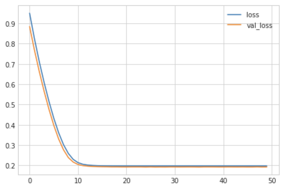
It’s not uncommon for the curves to follow a “hockey stick” pattern like you see here. This makes the final part of training hard to see, so let’s start at epoch 10 instead:
# Start the plot at epoch 10
history_df.loc[10:, ['loss', 'val_loss']].plot()
print("Minimum Validation Loss: {:0.4f}".format(history_df['val_loss'].min()));
Minimum Validation Loss: 0.1923
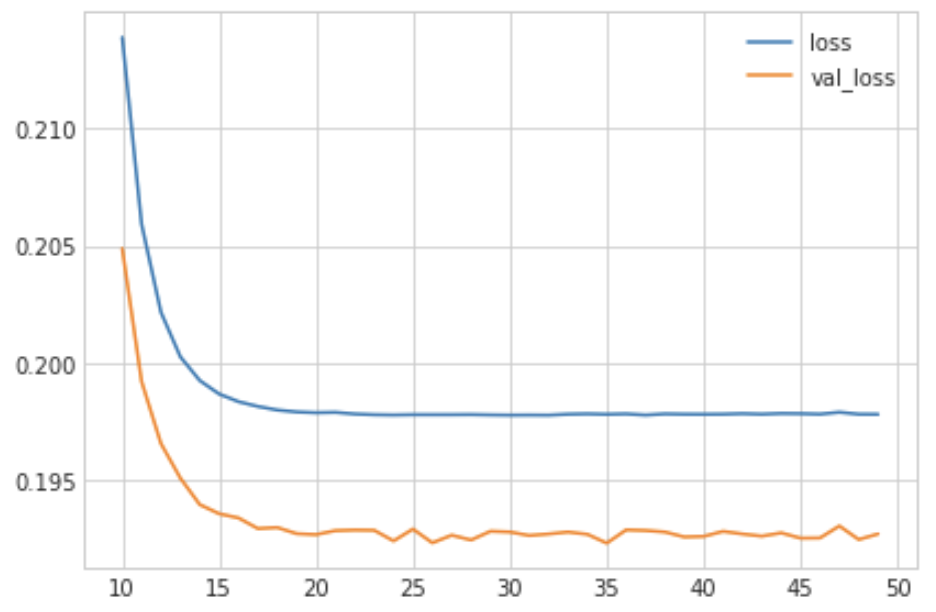
The gap between these curves is quite small and the validation loss never increases, so it’s more likely that the network is underfitting than overfitting. It would be worth experimenting with more capacity to see if that’s the case.
Now let’s add some capacity to our network. We’ll add three hidden layers with 128 units each. Run the next cell to train the network and see the learning curves.
model = keras.Sequential([
    layers.Dense(128, activation='relu', input_shape=input_shape),
    layers.Dense(64, activation='relu'),
    layers.Dense(1)
])
model.compile(
    optimizer='adam',
    loss='mae',
)
history = model.fit(
    X_train, y_train,
    validation_data=(X_valid, y_valid),
    batch_size=512,
    epochs=50,
)
history_df = pd.DataFrame(history.history)
history_df.loc[:, ['loss', 'val_loss']].plot()
print("Minimum Validation Loss: {:0.4f}".format(history_df['val_loss'].min()));
Minimum Validation Loss: 0.1934
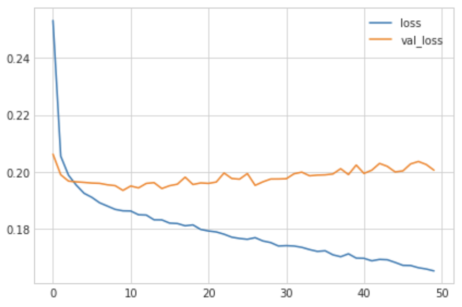
Now the validation loss begins to rise very early, while the training loss continues to decrease. This indicates that the network has begun to overfit. At this point, we would need to try something to prevent it, either by reducing the number of units or through a method like early stopping.
Now define an early stopping callback that waits 5 epochs (‘patience’) for a change in validation loss of at least 0.001 (min_delta) and keeps the weights with the best loss (restore_best_weights).
from tensorflow.keras import callbacks

# Define an early stopping callback
early_stopping = callbacks.EarlyStopping(
    patience=5,
    min_delta=0.001,
    restore_best_weights=True,
)
Now train the model and get the learning curves. Notice the callbacks argument in model.fit.
model = keras.Sequential([
    layers.Dense(128, activation='relu', input_shape=input_shape),
    layers.Dense(64, activation='relu'),
    layers.Dense(1)
])
model.compile(
    optimizer='adam',
    loss='mae',
)
history = model.fit(
    X_train, y_train,
    validation_data=(X_valid, y_valid),
    batch_size=512,
    epochs=50,
    callbacks=[early_stopping]
)
history_df = pd.DataFrame(history.history)
history_df.loc[:, ['loss', 'val_loss']].plot()
print("Minimum Validation Loss: {:0.4f}".format(history_df['val_loss'].min()));
Minimum Validation Loss: 0.1930
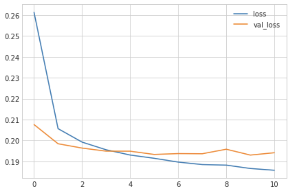
The early stopping callback did stop the training once the network began overfitting. Moreover, by including restore_best_weights we still get to keep the model where validation loss was lowest.
Try experimenting with patience and min_delta to see what difference it might make.