Sentiment Analysis of Reviews

Each review is labelled with either Pos or Neg to indicate whether the review has been assessed as positive or negative in the sentiment it expresses. You should treat these labels as a reliable indicator of sentiment. You can assume that there are no neutral reviews. There are 1,382 reviews in the CSV file in total, 691 of which are positive and 691 of which are negative.

The Task

In a Jupyter notebook, implement a Naïve Bayes classifier using 80% (1106) of the reviews as training data. The training data should be selected at random from the full dataset. Test your classifier using the remaining 20% (276) of the reviews and report the classifier’s performance using a confusion matrix. It is important that you avoid issues of data leakage, meaning that your classifier should only be trained using data that it has access to from within the training data set. If there are words that only appear in the test data they should not be part of the classifier. You will need to make sure that your code is able to deal with encountering words in the test data that the classifier has not seen in the training data. It is up to you to decide how you will handle this. Your code will need to read the review data CSV file provided.

You will need to perform some clean up of the data before using it in your classifier. This should include:

• Identifying and excluding all punctuation and words that are not likely to affect sentiment (e.g. stopwords). As an example, Natural Language Toolkit (NLTK) in Python has lists of common stopwords that you may wish to use, but you are also free to find and use other libraries or tools for this.
• Ensuring that remaining words are not case sensitive (i.e. the classifier should not distinguish upper/lower case characters).

Your sentiment classifier should use a bag of words technique, in which you build a vocabulary of individual words that appear in the dataset once it has been cleaned up. You should attempt to treat minor variations of a word (e.g. ‘fault’, ‘faults’ and ‘faulty’) as instances of the same word (e.g. ‘fault’) when you are using them in your classifier. You should investigate and implement stemming as a way of doing this.

For each review you should create a vector as input for your classifier, containing EITHER binary values indicating whether a word/stem occurs in the review OR a numerical count of the number of times each word/stem appears. As described above, vectors that are used to train the classifier should only include words that appear in the training data (and not words that only exist within the test data). Note: You do not need to code everything required from scratch. For this lab exercise you are encouraged to make use of existing libraries for all parts of the tasks. For example, you may find the MultinomialNB classifier in scikit.learn and natural language processing tools such as NLTK and spaCy useful for this task. It is also important to note that there is no single correct answer in terms of the output and performance of your classifier. This will depend on the choices you make about how you deal with the data at each stage of the process – your markers will not be looking for a specific level of performance, rather that you have taken appropriate steps and implemented them correctly.

import pandas as pd
import numpy as np
import pickle

import nltk
from nltk.corpus import stopwords
from nltk.stem import PorterStemmer

from tqdm import tqdm
tqdm.pandas()

from collections import Counter
import string

from sklearn.model_selection import train_test_split
from sklearn.naive_bayes import MultinomialNB, ComplementNB
from sklearn.model_selection import KFold
from sklearn.model_selection import GridSearchCV
from sklearn.feature_extraction.text import CountVectorizer
from sklearn.feature_extraction.text import TfidfVectorizer
from sklearn.feature_extraction import DictVectorizer
from sklearn.metrics import classification_report
from sklearn.metrics import confusion_matrix, plot_confusion_matrix

import seaborn as sns
import matplotlib.pyplot as plt
%config InlineBackend.figure_format = 'retina'
sns.set_style("dark")

Text Analysis is a major application field for machine learning algorithms. However the raw data, a sequence of symbols cannot be fed directly to the algorithms themselves as most of them expect numerical feature vectors with a fixed size rather than the raw text documents with variable length.

In order to address this, scikit-learn provides utilities for the most common ways to extract numerical features from text content, namely:

• Tokenizing strings and giving an integer id for each possible token, for instance by using white-spaces and punctuation as token separators.

• Counting the occurrences of tokens in each document.

• Normalizing and weighting with diminishing importance tokens that occur in the majority of samples / documents.

In this scheme, features and samples are defined as follows:

• Each individual token occurrence frequency (normalized or not) is treated as a feature.

• The vector of all the token frequencies for a given document is considered a multivariate sample.

A corpus of documents can thus be represented by a matrix with one row per document and one column per token (e.g. word) occurring in the corpus.

We call vectorization the general process of turning a collection of text documents into numerical feature vectors. This specific strategy (tokenization, counting and normalization) is called the Bag of Words or “Bag of n-grams” representation. Documents are described by word occurrences while completely ignoring the relative position information of the words in the document.

Stop words are words like “and”, “the”, “him”, which are presumed to be uninformative in representing the content of a text, and which may be removed to avoid them being construed as signal for prediction. Sometimes, however, similar words are useful for prediction, such as in classifying writing style or personality.

Preprocessing

Steps Taken:

• Remove Punctuation and Digits and make lowercase, Remove words < len(3)
• Tokenize the words, and remove stopwords
• Stem the words

def process_text(filename):
    df = pd.read_csv(filename)
    stop_words = stopwords.words('english')
    # Remove Punctuation and Digits and make lowercase, Remove words < len(3)
    list_of_chars_and_digits = string.punctuation + string.digits
    df['remove_punc_and_digits'] = df['Review'].str.replace(f"[{list_of_chars_and_digits}]", " ", regex=True).apply(str.lower).str.findall("\w{3,}").str.join(" ")

    # Tokenize the words, and remove stopwords
    df['word_tokens'] = df['remove_punc_and_digits'].apply(nltk.word_tokenize)
    df['remove_stopwords'] = df['word_tokens'].apply(lambda x: [word for word in x if word not in stop_words]) 
    df['remove_stopwords_count'] = df['remove_stopwords'].apply(Counter)
    
    # Stem the words
    ps = PorterStemmer()
    df['stemmed'] = df['remove_stopwords'].apply(lambda x: [ps.stem(word) for word in x])
    df['stemmed_count'] = df['stemmed'].apply(Counter)
    
    # Final processed sentence
    df['stemmed_sentence'] = df['stemmed'].str.join(' ')
    return df

df = process_text('car_reviews.csv')
df

	Sentiment	Review	remove_punc_and_digits	word_tokens	remove_stopwords	remove_stopwords_count	stemmed	stemmed_count	stemmed_sentence
0	Neg	In 1992 we bought a new Taurus and we really ...	bought new taurus and really loved decided try...	[bought, new, taurus, and, really, loved, deci...	[bought, new, taurus, really, loved, decided, ...	{'bought': 2, 'new': 3, 'taurus': 3, 'really':...	[bought, new, tauru, realli, love, decid, tri,...	{'bought': 2, 'new': 3, 'tauru': 3, 'realli': ...	bought new tauru realli love decid tri new tau...
1	Neg	The last business trip I drove to San Franci...	the last business trip drove san francisco wen...	[the, last, business, trip, drove, san, franci...	[last, business, trip, drove, san, francisco, ...	{'last': 1, 'business': 2, 'trip': 7, 'drove':...	[last, busi, trip, drove, san, francisco, went...	{'last': 1, 'busi': 2, 'trip': 7, 'drove': 1, ...	last busi trip drove san francisco went hertz ...
2	Neg	My husband and I purchased a 1990 Ford F250 a...	husband and purchased ford and had nothing but...	[husband, and, purchased, ford, and, had, noth...	[husband, purchased, ford, nothing, problems, ...	{'husband': 1, 'purchased': 1, 'ford': 2, 'not...	[husband, purchas, ford, noth, problem, own, v...	{'husband': 1, 'purchas': 1, 'ford': 2, 'noth'...	husband purchas ford noth problem own vehicl a...
3	Neg	I feel I have a thorough opinion of this truc...	feel have thorough opinion this truck compared...	[feel, have, thorough, opinion, this, truck, c...	[feel, thorough, opinion, truck, compared, pos...	{'feel': 1, 'thorough': 1, 'opinion': 1, 'truc...	[feel, thorough, opinion, truck, compar, post,...	{'feel': 1, 'thorough': 1, 'opinion': 1, 'truc...	feel thorough opinion truck compar post evalu ...
4	Neg	AS a mother of 3 all of whom are still in ca...	mother all whom are still carseats the only lo...	[mother, all, whom, are, still, carseats, the,...	[mother, still, carseats, logical, thing, trad...	{'mother': 1, 'still': 1, 'carseats': 1, 'logi...	[mother, still, carseat, logic, thing, trade, ...	{'mother': 1, 'still': 1, 'carseat': 1, 'logic...	mother still carseat logic thing trade minivan...
...	...	...	...	...	...	...	...	...	...
1377	Pos	In June we bought the Sony Limited Edition Fo...	june bought the sony limited edition focus sed...	[june, bought, the, sony, limited, edition, fo...	[june, bought, sony, limited, edition, focus, ...	{'june': 1, 'bought': 2, 'sony': 6, 'limited':...	[june, bought, soni, limit, edit, focu, sedan,...	{'june': 1, 'bought': 2, 'soni': 6, 'limit': 4...	june bought soni limit edit focu sedan simpli ...
1378	Pos	After 140 000 miles we decided to replace my...	after miles decided replace wife toyota camry ...	[after, miles, decided, replace, wife, toyota,...	[miles, decided, replace, wife, toyota, camry,...	{'miles': 1, 'decided': 1, 'replace': 1, 'wife...	[mile, decid, replac, wife, toyota, camri, fou...	{'mile': 1, 'decid': 1, 'replac': 2, 'wife': 2...	mile decid replac wife toyota camri found new ...
1379	Pos	The Ford Focus is a great little record setti...	the ford focus great little record setting car...	[the, ford, focus, great, little, record, sett...	[ford, focus, great, little, record, setting, ...	{'ford': 4, 'focus': 4, 'great': 4, 'little': ...	[ford, focu, great, littl, record, set, car, f...	{'ford': 4, 'focu': 4, 'great': 4, 'littl': 2,...	ford focu great littl record set car first car...
1380	Pos	I needed a new car because my hyundai excel 9...	needed new car because hyundai excel had decid...	[needed, new, car, because, hyundai, excel, ha...	[needed, new, car, hyundai, excel, decided, sh...	{'needed': 1, 'new': 1, 'car': 14, 'hyundai': ...	[need, new, car, hyundai, excel, decid, shop, ...	{'need': 2, 'new': 1, 'car': 15, 'hyundai': 1,...	need new car hyundai excel decid shop around n...
1381	Pos	The 2000 Ford Focus SE 4 door sedan has a spa...	the ford focus door sedan has spacious interio...	[the, ford, focus, door, sedan, has, spacious,...	[ford, focus, door, sedan, spacious, interior,...	{'ford': 2, 'focus': 10, 'door': 2, 'sedan': 1...	[ford, focu, door, sedan, spaciou, interior, s...	{'ford': 2, 'focu': 10, 'door': 2, 'sedan': 1,...	ford focu door sedan spaciou interior solid fe...

1382 rows × 9 columns

print('Review unprocessed:\n')
print(f"{df['Review'][0]}\n")
print('Remove punctuation, digits, short words and make lowercase:\n')
print(f"{df['remove_punc_and_digits'][0]}\n")
print('Tokenized words:\n')
print(f"{df['word_tokens'][0]}\n")
print('Stopwords removed:\n')
print(f"{df['remove_stopwords'][0]}\n")
print('Stemmed words:\n')
print(f"{df['stemmed'][0]}\n")
print('Review fully processed:\n')
print(f"{df['stemmed_sentence'][0]}\n")

Review unprocessed:

 In 1992 we bought a new Taurus and we really loved it  So in 1999 we decided to try a new Taurus  I did not care for the style of the newer version  but bought it anyway I do not like the new car half as much as i liked our other one  Thee dash is much to deep and takes up a lot of room  I do not find the seats as comfortable and the way the sides stick out further than the strip that should protect your card from denting It drives nice and has good pick up  But you can not see the hood at all from the driver seat and judging and parking is difficult  It has a very small gas tank I would not buy a Taurus if I had it to do over  I would rather have my 1992 back  I don t think the style is as nice as the the 1992  and it was a mistake to change the style  In less than a month we had a dead battery and a flat tire 

Remove punctuation, digits, short words and make lowercase:

bought new taurus and really loved decided try new taurus did not care for the style the newer version but bought anyway not like the new car half much liked our other one thee dash much deep and takes lot room not find the seats comfortable and the way the sides stick out further than the strip that should protect your card from denting drives nice and has good pick but you can not see the hood all from the driver seat and judging and parking difficult has very small gas tank would not buy taurus had over would rather have back don think the style nice the the and was mistake change the style less than month had dead battery and flat tire

Tokenized words:

['bought', 'new', 'taurus', 'and', 'really', 'loved', 'decided', 'try', 'new', 'taurus', 'did', 'not', 'care', 'for', 'the', 'style', 'the', 'newer', 'version', 'but', 'bought', 'anyway', 'not', 'like', 'the', 'new', 'car', 'half', 'much', 'liked', 'our', 'other', 'one', 'thee', 'dash', 'much', 'deep', 'and', 'takes', 'lot', 'room', 'not', 'find', 'the', 'seats', 'comfortable', 'and', 'the', 'way', 'the', 'sides', 'stick', 'out', 'further', 'than', 'the', 'strip', 'that', 'should', 'protect', 'your', 'card', 'from', 'denting', 'drives', 'nice', 'and', 'has', 'good', 'pick', 'but', 'you', 'can', 'not', 'see', 'the', 'hood', 'all', 'from', 'the', 'driver', 'seat', 'and', 'judging', 'and', 'parking', 'difficult', 'has', 'very', 'small', 'gas', 'tank', 'would', 'not', 'buy', 'taurus', 'had', 'over', 'would', 'rather', 'have', 'back', 'don', 'think', 'the', 'style', 'nice', 'the', 'the', 'and', 'was', 'mistake', 'change', 'the', 'style', 'less', 'than', 'month', 'had', 'dead', 'battery', 'and', 'flat', 'tire']

Stopwords removed:

['bought', 'new', 'taurus', 'really', 'loved', 'decided', 'try', 'new', 'taurus', 'care', 'style', 'newer', 'version', 'bought', 'anyway', 'like', 'new', 'car', 'half', 'much', 'liked', 'one', 'thee', 'dash', 'much', 'deep', 'takes', 'lot', 'room', 'find', 'seats', 'comfortable', 'way', 'sides', 'stick', 'strip', 'protect', 'card', 'denting', 'drives', 'nice', 'good', 'pick', 'see', 'hood', 'driver', 'seat', 'judging', 'parking', 'difficult', 'small', 'gas', 'tank', 'would', 'buy', 'taurus', 'would', 'rather', 'back', 'think', 'style', 'nice', 'mistake', 'change', 'style', 'less', 'month', 'dead', 'battery', 'flat', 'tire']

Stemmed words:

['bought', 'new', 'tauru', 'realli', 'love', 'decid', 'tri', 'new', 'tauru', 'care', 'style', 'newer', 'version', 'bought', 'anyway', 'like', 'new', 'car', 'half', 'much', 'like', 'one', 'thee', 'dash', 'much', 'deep', 'take', 'lot', 'room', 'find', 'seat', 'comfort', 'way', 'side', 'stick', 'strip', 'protect', 'card', 'dent', 'drive', 'nice', 'good', 'pick', 'see', 'hood', 'driver', 'seat', 'judg', 'park', 'difficult', 'small', 'ga', 'tank', 'would', 'buy', 'tauru', 'would', 'rather', 'back', 'think', 'style', 'nice', 'mistak', 'chang', 'style', 'less', 'month', 'dead', 'batteri', 'flat', 'tire']

Review fully processed:

bought new tauru realli love decid tri new tauru care style newer version bought anyway like new car half much like one thee dash much deep take lot room find seat comfort way side stick strip protect card dent drive nice good pick see hood driver seat judg park difficult small ga tank would buy tauru would rather back think style nice mistak chang style less month dead batteri flat tire

print('Stopwords count:\n')
print(f"{df['remove_stopwords_count'][0]}\n")
print('Stemmed count:\n')
print(f"{df['stemmed_count'][0]}\n")

Stopwords count:

Counter({'new': 3, 'taurus': 3, 'style': 3, 'bought': 2, 'much': 2, 'nice': 2, 'would': 2, 'really': 1, 'loved': 1, 'decided': 1, 'try': 1, 'care': 1, 'newer': 1, 'version': 1, 'anyway': 1, 'like': 1, 'car': 1, 'half': 1, 'liked': 1, 'one': 1, 'thee': 1, 'dash': 1, 'deep': 1, 'takes': 1, 'lot': 1, 'room': 1, 'find': 1, 'seats': 1, 'comfortable': 1, 'way': 1, 'sides': 1, 'stick': 1, 'strip': 1, 'protect': 1, 'card': 1, 'denting': 1, 'drives': 1, 'good': 1, 'pick': 1, 'see': 1, 'hood': 1, 'driver': 1, 'seat': 1, 'judging': 1, 'parking': 1, 'difficult': 1, 'small': 1, 'gas': 1, 'tank': 1, 'buy': 1, 'rather': 1, 'back': 1, 'think': 1, 'mistake': 1, 'change': 1, 'less': 1, 'month': 1, 'dead': 1, 'battery': 1, 'flat': 1, 'tire': 1})

Stemmed count:

Counter({'new': 3, 'tauru': 3, 'style': 3, 'bought': 2, 'like': 2, 'much': 2, 'seat': 2, 'nice': 2, 'would': 2, 'realli': 1, 'love': 1, 'decid': 1, 'tri': 1, 'care': 1, 'newer': 1, 'version': 1, 'anyway': 1, 'car': 1, 'half': 1, 'one': 1, 'thee': 1, 'dash': 1, 'deep': 1, 'take': 1, 'lot': 1, 'room': 1, 'find': 1, 'comfort': 1, 'way': 1, 'side': 1, 'stick': 1, 'strip': 1, 'protect': 1, 'card': 1, 'dent': 1, 'drive': 1, 'good': 1, 'pick': 1, 'see': 1, 'hood': 1, 'driver': 1, 'judg': 1, 'park': 1, 'difficult': 1, 'small': 1, 'ga': 1, 'tank': 1, 'buy': 1, 'rather': 1, 'back': 1, 'think': 1, 'mistak': 1, 'chang': 1, 'less': 1, 'month': 1, 'dead': 1, 'batteri': 1, 'flat': 1, 'tire': 1})

Train Test Split the Data

# Sentiment target, convert to 1 for pos, 0 for neg
y = df['Sentiment'].map({'Pos': 1, 'Neg': 0})
# Fully processed sentence
X = df['stemmed_sentence']

# Break off validation set from training data
X_train, X_test, y_train, y_test = train_test_split(X, y, 
                                        train_size=0.8, test_size=0.2,
                                        random_state=0)
X_test

655     admit much mechan detail technic get basic six...
975     ford made littl buzz fact current ford mustang...
445     ford mustang realli made great car new convert...
610     write review kind truck less accid fate rent o...
459     ever one optic illus book pictur look like old...
                              ...                        
744     truck purchas review ford supercrew offroad pa...
764     famili two aerostar love three kid need extra ...
1149    got one liter engin liter pzev engin late car ...
758     everi year two decid time purchas new car wife...
251     dislik ford ranger purchas ford ranger super c...
Name: stemmed_sentence, Length: 277, dtype: object

Bag of Words

The bag-of-words model is very simple to understand and implement and offers a lot of flexibility for customization on your specific text data.

It has been used with great success on prediction problems like language modeling and documentation classification.

Nevertheless, it suffers from some shortcomings, such as:

• Vocabulary: The vocabulary requires careful design, most specifically in order to manage the size, which impacts the sparsity of the document representations.
• Sparsity: Sparse representations are harder to model both for computational reasons (space and time complexity) and also for information reasons, where the challenge is for the models to harness so little information in such a large representational space.
• Meaning: Discarding word order ignores the context, and in turn meaning of words in the document (semantics). Context and meaning can offer a lot to the model, that if modeled could tell the difference between the same words differently arranged (“this is interesting” vs “is this interesting”), synonyms (“old bike” vs “used bike”), and much more.

Avoiding Data Leakage

• fit_transform() is used on the training data so that we can scale the training data and also learn the transformation parameters of that data. These learned parameters are then used to transform our test data.

• Using the transform() method we can use the same transformation calculated from our training data to transform our test data. Thus, the parameters learned by our model using the training data will help us to transform our test data. In this case, out of vocabulary words are avoided.

More about the difference between fit_transform() and transform() can be found here.

vect = CountVectorizer()

# Fit the training set, note the different class methods for transform between train and test.
X_train_bow = vect.fit_transform(X_train)

# Transform method only to ensure no Data Leakage to the training set.
X_test_bow = vect.transform(X_test)

# Display first 15 word count pairs
{k: vect.vocabulary_[k] for k in list(vect.vocabulary_)[:15]}

{'cobra': 1408,
 'second': 6635,
 'particular': 5443,
 'breed': 878,
 'own': 5380,
 'first': 2854,
 'convert': 1623,
 'initi': 3887,
 'reaction': 6083,
 'saw': 6558,
 'reveal': 6341,
 'car': 1080,
 'wow': 8791,
 'statist': 7288,
 'alon': 214}

Confusion Matrix for MultinomialNB()

Classification report explained:

• The recall means “how many of this class you find over the whole number of elements of this class”
• The precision will be “how many are correctly classified among that class”
• The f1-score is the harmonic mean between precision & recall
• The support is the number of occurence of the given class in your dataset
• 0 stands for ‘Negative’
• 1 stands for ‘Positive’

Confusion Matrix: \(\begin{bmatrix} TN & FP \\ FN & TP \end{bmatrix}\)

The best confusion matrix has a low:

• False Positive: You predicted positive and it’s false. (Type 1 Error)
• False Negative: You predicted negative and it’s false. (Type 2 Error)

and a high:

• True Positive: You predicted positive and it’s true.
• True Negative: You predicted negative and it’s true.

Essentially you want most of your values to lie along the trace of the matrix.

def matrix(X_train,y_train,X_test,y_test, alpha=10):

    # Run the model on the training set
    model = MultinomialNB(alpha=alpha)
    model.fit(X_train, y_train)

    # Test the model with the test set
    predict = model.predict(X_test)

    # Save the model
    # pickle.dump(model, open('model.pkl','wb'))

    # Define the confusion matrix
    conf_mat = confusion_matrix(y_test, predict)
    print('Confusion Matrix:\n')
    print(conf_mat)

    # Get the classification report
    report = classification_report(y_test,predict)
    print(report)
    
    fig, ax = plt.subplots(figsize=(10, 10))
    plot_confusion_matrix(model, X_test, y_test, ax=ax)

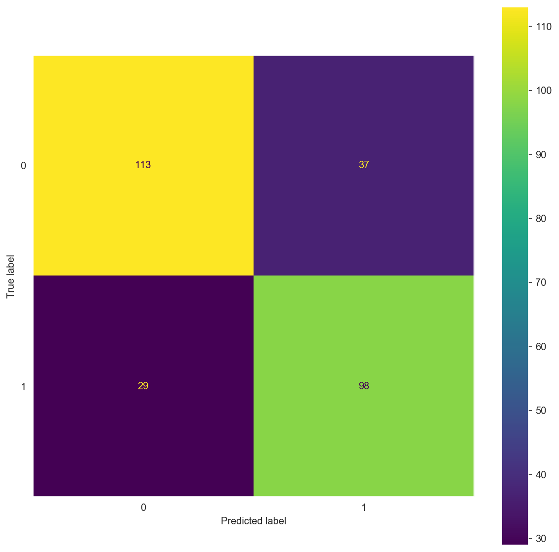
matrix(X_train_bow, y_train, X_test_bow, y_test)

Confusion Matrix:

[[113  37]
 [ 29  98]]
              precision    recall  f1-score   support

           0       0.80      0.75      0.77       150
           1       0.73      0.77      0.75       127

    accuracy                           0.76       277
   macro avg       0.76      0.76      0.76       277
weighted avg       0.76      0.76      0.76       277

Top Features

def top_features():
    # Run the model
    model = MultinomialNB()
    model.fit(X_train_bow, y_train)
    
    # Get the top 10 pos 
    feature_names = vect.get_feature_names()
    a = getattr(model, 'feature_log_prob_')
    top_pos = list(zip(a[1], feature_names))
    top_pos.sort(key=lambda x: x[0])
    l = len(top_pos)
    print('\nThe Top 10 Positive Class Features are:\n')
    for i in range(1,11):
        print(top_pos[l-i][1])
    
    # Get the top 10 neg 
    top_neg = list(zip(a[0], feature_names))
    top_neg.sort(key=lambda x: x[0])
    l = len(top_neg)
    print('\nThe Top 10 Negative Class Features are:\n')
    for i in range(1,11):
        print(top_neg[l-i][1])

top_features()

The Top 10 Positive Class Features are:

car
ford
drive
seat
like
truck
one
get
vehicl
look

The Top 10 Negative Class Features are:

car
ford
like
problem
get
drive
one
vehicl
seat
would

Improve the Model

Identify and research a way to improve on the solution, such that you would expect to do better at classifying the sentiment of the reviews. You may either:

• Identify an alternative classification algorithm, or
• Apply modifications to the Naïve Bayes implementation, for example trying different classification of different size n-grams (multi-word phrases). Implement this improvement and compare the results to your initial Naïve Bayes classifier.

Plans for Improvement

• The first step to improve a model is the correct choice of hyperparameters. Using the KFold() and GridSearch() classes we can optimise the various parameters associated with the model MultinomialNB(). Naive Bayes models only have the alpha parameter to optimise, so we begin across a range of values.
• Other factors such as word vectorising in the pre-processing stage, rather than the bag of words approach could yield different results.
• Using DictVectorizer() could also improve the model, from the stemmed_counts column in preprocessing.
• TfidVectorizer() is likely to vastly improve the model.
• Words which appear only once don’t help classification at all, if only because they can never be matched again. More generally, words which appear rarely are more likely to appear by chance, so using them as features causes overfitting.

Hyperparameter Tuning using KFold() and GridSearch()

Implemented improvements:

• Hyperparameter tuning for \( \alpha \).

We use the KFold() and GridSearch() to find the optimal \( \alpha \) value for our model.

def param_tuning(X_train):
    # K-fold cross validation
    cv = KFold(n_splits=5) 
    model = MultinomialNB()
    # Hyperparameters
    parameters = {'alpha':alpha_values}
    # Gridsearch
    clf = GridSearchCV(model, parameters, cv=cv, scoring='roc_auc', return_train_score=True, verbose=1)
    # Fit the Model
    clf.fit(X_train, y_train)
    return clf

alpha_values = [0.00001, 0.0001, 0.001,0.01, 0.1, 1, 10, 100, 1000, 10000, 100000]
clf = param_tuning(X_train_bow)
# Extract stats for plotting
train_auc = clf.cv_results_['mean_train_score']
train_auc_std = clf.cv_results_['std_train_score']
cv_auc = clf.cv_results_['mean_test_score'] 
cv_auc_std = clf.cv_results_['std_test_score']
best_alpha = clf.best_params_['alpha']

Fitting 5 folds for each of 11 candidates, totalling 55 fits

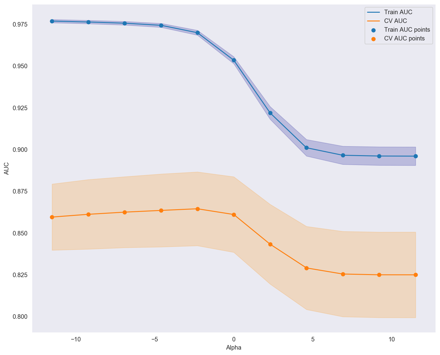
Below is a plot displaying all of the respective K-folds and fitted \( \alpha \) values, with the best \( \alpha \) value obtained around \( 1 \).

def plot_error():
    alpha_values_lst = [np.log(x) for x in alpha_values]

    plt.subplots(figsize=(12,10))
    plt.plot(alpha_values_lst, train_auc, label='Train AUC')
    plt.gca().fill_between(alpha_values_lst,train_auc - train_auc_std,train_auc + train_auc_std,alpha=0.2,color='darkblue')

    plt.plot(alpha_values_lst, cv_auc, label='CV AUC')
    plt.gca().fill_between(alpha_values_lst,cv_auc - cv_auc_std,cv_auc + cv_auc_std,alpha=0.2,color='darkorange')

    plt.scatter(alpha_values_lst, train_auc, label='Train AUC points')
    plt.scatter(alpha_values_lst, cv_auc, label='CV AUC points')

    plt.legend()
    plt.xlabel("Alpha")
    plt.ylabel("AUC")
    plt.show()

    print("Best cross-validation score: {:.3f}".format(clf.best_score_))
    print('The best alpha from gridsearch :',best_alpha)

plot_error()

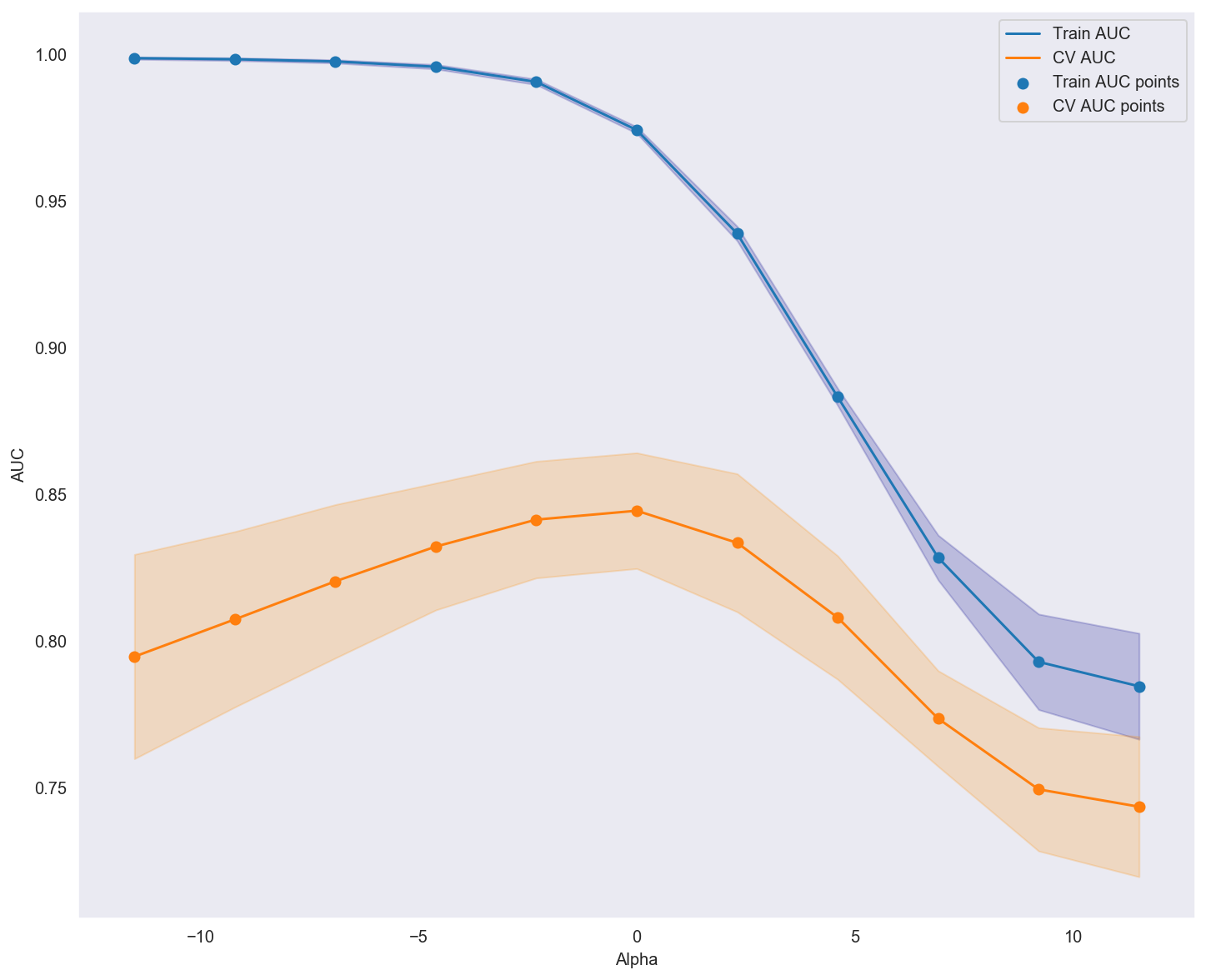
Best cross-validation score: 0.844
The best alpha from gridsearch : 1

Confusion Matrix (alpha=1)

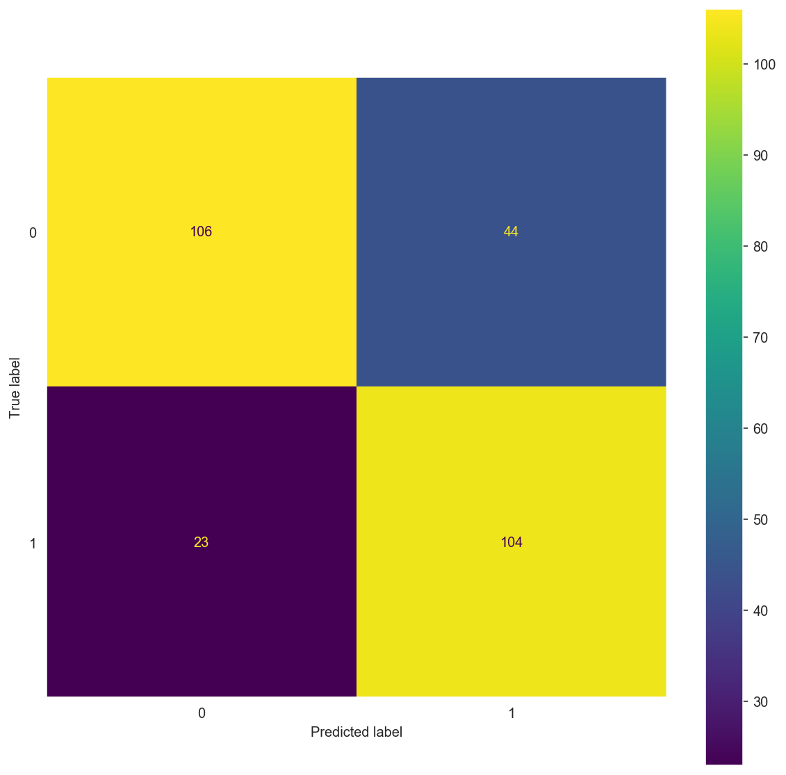
matrix(X_train_bow, y_train, X_test_bow, y_test, alpha=1)

Confusion Matrix:

[[106  44]
 [ 23 104]]
              precision    recall  f1-score   support

           0       0.82      0.71      0.76       150
           1       0.70      0.82      0.76       127

    accuracy                           0.76       277
   macro avg       0.76      0.76      0.76       277
weighted avg       0.77      0.76      0.76       277

Preprocessing Improvement with Hyperparameter Tuning (Bag of Words)

Implemented improvements:

• Preprocessed stemmed words with \( N \) occurrences dropped.
• Hyperparameter tuning for \( \alpha \).

Naive Bayes Considerations

• Naive Bayes is very sensitive to overfitting since it considers all the features independently of each other.
• It’s also quite likely that the final number of features (words) is too high with respect to the number of instances. A low ratio instances/words causes overfitting. The solution is to filter out words which occur less than \( N \) times in the data. Maybe try with several values of \( N \), starting with \( N=2 \).

def remove_word_occurrences(df, N=2):
    # Extra reduction step to remove words that occur less than N times.
    total_rows = len(df)
    df['reduced_stem_count'] = [{k:v for k,v in df['stemmed_count'][row].items() if v > N} for row in range(total_rows)]
    df['reduced_stemmed'] = [[k for k in df['reduced_stem_count'][row]] for row in range(total_rows)]
    df['reduced_stemmed_sentence'] = [' '.join(i) for i in df['reduced_stemmed']]
    return df

df = process_text('car_reviews.csv')
df = remove_word_occurrences(df, N=2)


df['reduced_stemmed_sentence'][:5]

0                                      new tauru style
1           trip tauru comfort seat uncomfort car long
2    problem vehicl time shop took day found mechan...
3    truck vehicl mile mainten never problem found ...
4                vehicl fact van car way like windstar
Name: reduced_stemmed_sentence, dtype: object

df['stemmed_sentence'][:5]

0    bought new tauru realli love decid tri new tau...
1    last busi trip drove san francisco went hertz ...
2    husband purchas ford noth problem own vehicl a...
3    feel thorough opinion truck compar post evalu ...
4    mother still carseat logic thing trade minivan...
Name: stemmed_sentence, dtype: object

# Sentiment target, convert to 1 for pos, 0 for neg
y = df['Sentiment'].replace('Pos', 1).replace('Neg', 0)
# Fully processed sentence
X = df['reduced_stemmed_sentence']

# Break off validation set from training data
X_train, X_test, y_train, y_test = train_test_split(X, y, 
                                        train_size=0.8, test_size=0.2,
                                        random_state=0)

vect = CountVectorizer()

# Data Leakage Prevention
X_train_bow = vect.fit_transform(X_train)
X_test_bow = vect.transform(X_test)

alpha_values = [0.00001,0.0001,0.001,0.01,0.1,1,10,100,1000,10000,100000]
clf = param_tuning(X_train_bow)
# defining train and cross_validation
train_auc = clf.cv_results_['mean_train_score']
train_auc_std = clf.cv_results_['std_train_score']
cv_auc = clf.cv_results_['mean_test_score'] 
cv_auc_std = clf.cv_results_['std_test_score']
best_alpha = clf.best_params_['alpha']

plot_error()

Fitting 5 folds for each of 11 candidates, totalling 55 fits

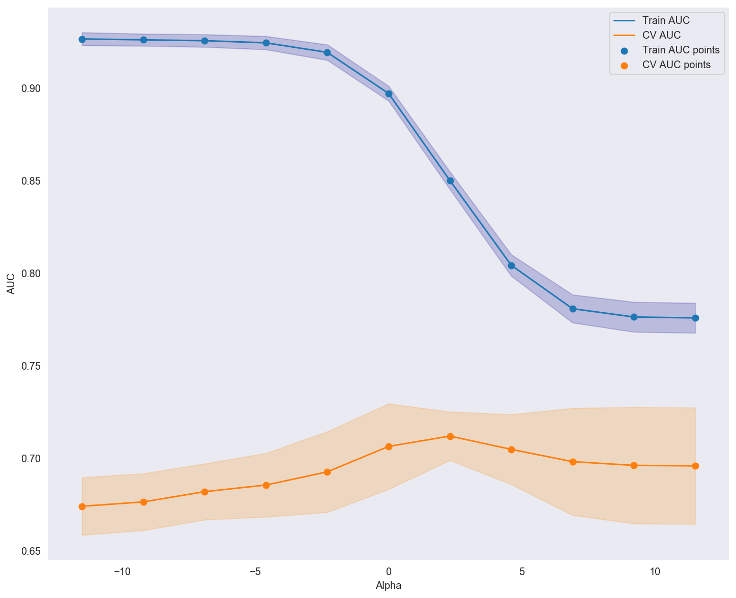
Best cross-validation score: 0.712
The best alpha from gridsearch : 10

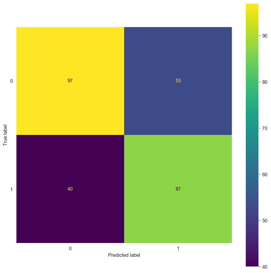
Confusion Matrix (alpha=10)

matrix(X_train_bow, y_train, X_test_bow, y_test, alpha=10)

Confusion Matrix:

[[97 53]
 [40 87]]
              precision    recall  f1-score   support

           0       0.71      0.65      0.68       150
           1       0.62      0.69      0.65       127

    accuracy                           0.66       277
   macro avg       0.66      0.67      0.66       277
weighted avg       0.67      0.66      0.66       277

Improvements Using TfidVectorizer()

A problem with scoring word frequency is that highly frequent words start to dominate in the document (e.g. larger score), but may not contain as much “informational content” to the model as rarer but perhaps domain specific words.

One approach is to rescale the frequency of words by how often they appear in all documents, so that the scores for frequent words like “the” that are also frequent across all documents are penalized.

This approach to scoring is called Term Frequency – Inverse Document Frequency, or TF-IDF for short, where:

• Term Frequency: is a scoring of the frequency of the word in the current document.
• Inverse Document Frequency: is a scoring of how rare the word is across documents. The scores are a weighting where not all words are equally as important or interesting.

The scores have the effect of highlighting words that are distinct (contain useful information) in a given document.

Implemented improvements:

• Preprocessed stemmed words with \( N \) occurrences dropped.
• Hyperparameter tuning for \( \alpha \).
• Use of the TfidVectorizer() instead of the CountVectorizer()

The sklearn class TfidVectorizer might have a small performance increase as opposed to the CountVectorizer (Bag of Words), which uses produces a sparse representation of the counts using scipy.sparse.csr_matrix.

# Sentiment target, convert to 1 for pos, 0 for neg
y_tf = df['Sentiment'].replace('Pos', 1).replace('Neg', 0)
# Fully processed sentence
X_tf = df['stemmed_sentence']

# Break off validation set from training data
X_train_tf, X_test_tf, y_train_tf, y_test_tf = train_test_split(X_tf, y_tf, 
                                        train_size=0.8, test_size=0.2,
                                        random_state=0)


tf_idf_vect = TfidfVectorizer(ngram_range=(1,2), min_df=10)
# Prevent data leakage
X_train_tf = tf_idf_vect.fit_transform(X_train_tf)
X_test_tf = tf_idf_vect.transform(X_test_tf)

alpha_values = [0.00001,0.0001,0.001,0.01,0.1,1,10,100,1000,10000,100000]
clf = param_tuning(X_train_tf)
# defining train and cross_validation
train_auc = clf.cv_results_['mean_train_score']
train_auc_std = clf.cv_results_['std_train_score']
cv_auc = clf.cv_results_['mean_test_score'] 
cv_auc_std = clf.cv_results_['std_test_score']
best_alpha = clf.best_params_['alpha']

plot_error()

Fitting 5 folds for each of 11 candidates, totalling 55 fits

Best cross-validation score: 0.865
The best alpha from gridsearch : 0.1

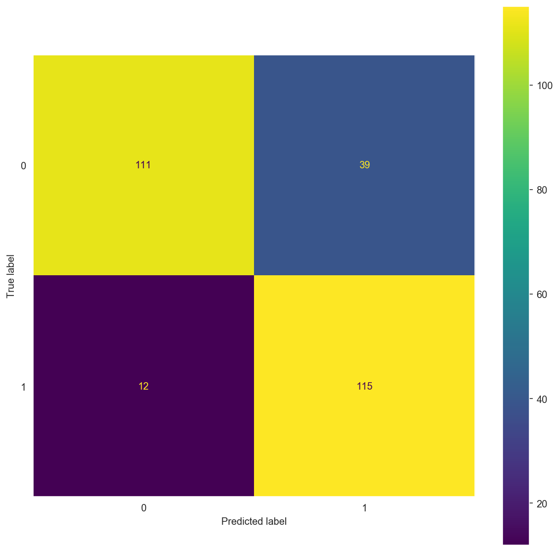
Confusion Matrix (\(\alpha=1)\)

matrix(X_train_tf, y_train_tf, X_test_tf, y_test_tf, alpha=0.1)

Confusion Matrix:

[[111  39]
 [ 12 115]]
              precision    recall  f1-score   support

           0       0.90      0.74      0.81       150
           1       0.75      0.91      0.82       127

    accuracy                           0.82       277
   macro avg       0.82      0.82      0.82       277
weighted avg       0.83      0.82      0.82       277

Using the ComplementNB() Model

Implemented potential improvements:

• Preprocessed stemmed words with \( N \) occurrences dropped.
• Hyperparameter tuning for \( \alpha \).
• Use of the TfidVectorizer() instead of the CountVectorizer()
• Use of the ComplementNB() instead of the MultiNomialNB()

ComplementNB() implements the complement naive Bayes (CNB) algorithm. CNB is an adaptation of the standard multinomial naive Bayes (MNB) algorithm that is particularly suited for imbalanced data sets. Specifically, CNB uses statistics from the complement of each class to compute the model’s weights. The inventors of CNB show empirically that the parameter estimates for CNB are more stable than those for MNB. Further, CNB regularly outperforms MNB (often by a considerable margin) on text classification tasks.

def matrix_comp(X_train,y_train,X_test,y_test):

    # Run the model on the training set
    model = ComplementNB(alpha=10)
    model.fit(X_train, y_train)

    # Test the model with the test set
    predict = model.predict(X_test)

    # Save the model
    pickle.dump(model, open('model.pkl','wb'))

    # Define the confusion matrix
    conf_mat = confusion_matrix(y_test, predict)
    print('Confusion Matrix:\n')
    print(conf_mat)

    # Get the classification report
    report = classification_report(y_test,predict)
    print(report)

    fig, ax = plt.subplots(figsize=(10, 10))
    plot_confusion_matrix(model, X_test, y_test, ax=ax)

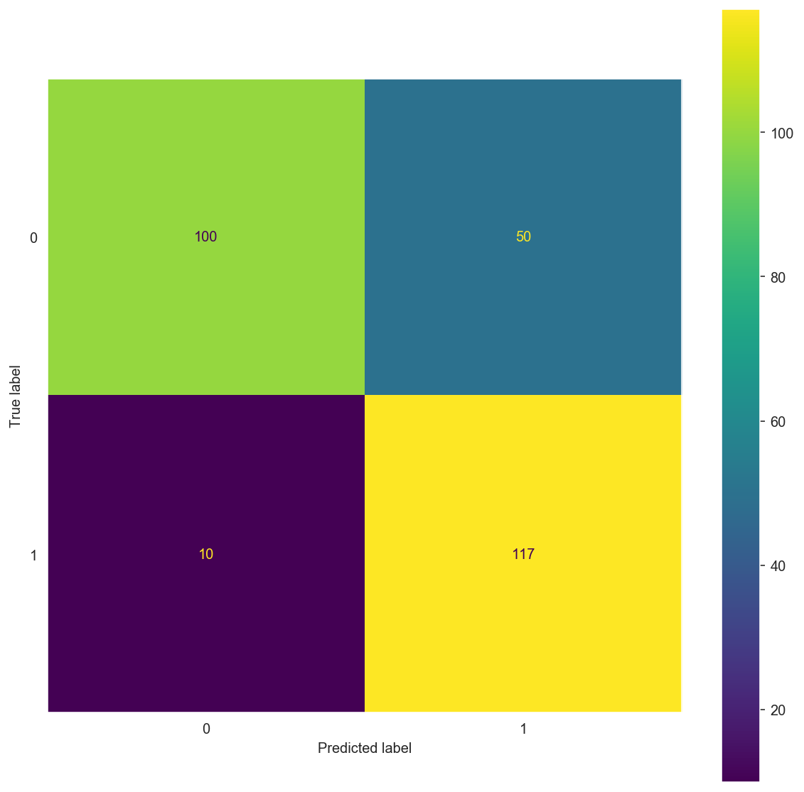
# Using Tfid
matrix_comp(X_train_tf, y_train_tf, X_test_tf, y_test_tf)
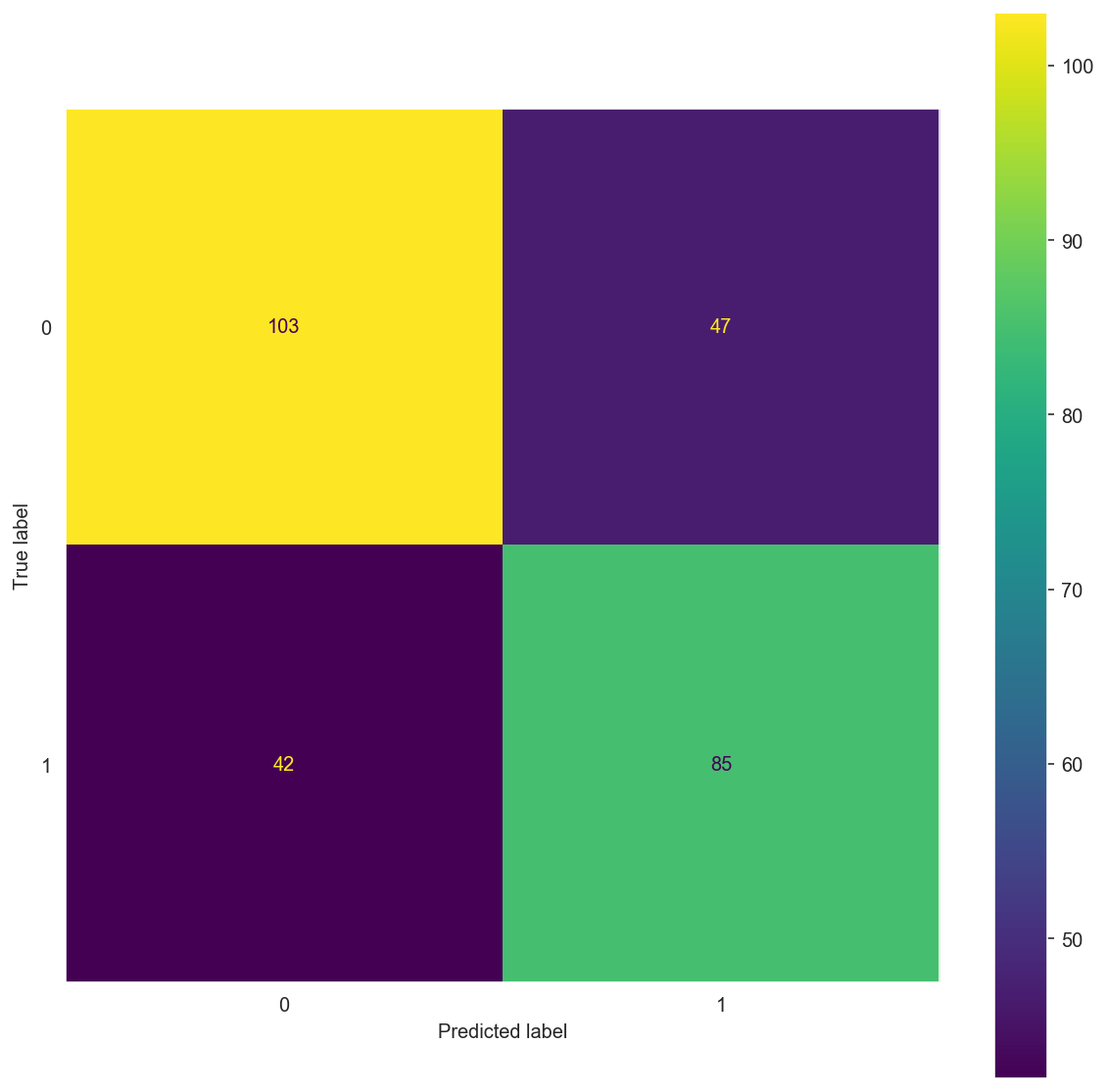
# Using Bag of Words
matrix_comp(X_train_bow, y_train, X_test_bow, y_test)

Confusion Matrix:

[[100  50]
 [ 10 117]]
              precision    recall  f1-score   support

           0       0.91      0.67      0.77       150
           1       0.70      0.92      0.80       127

    accuracy                           0.78       277
   macro avg       0.80      0.79      0.78       277
weighted avg       0.81      0.78      0.78       277

Confusion Matrix:

[[103  47]
 [ 42  85]]
              precision    recall  f1-score   support

           0       0.71      0.69      0.70       150
           1       0.64      0.67      0.66       127

    accuracy                           0.68       277
   macro avg       0.68      0.68      0.68       277
weighted avg       0.68      0.68      0.68       277

Using DictVectorizer()

Implemented potential improvements:

• Preprocessed stemmed words with \( N \) occurrences dropped.
• Hyperparameter tuning for \( \alpha \).
• Use of the DictVectorizer() instead of the CountVectorizer() and TfidVectorizer().
• Use of MultiNomialNB() for the model.

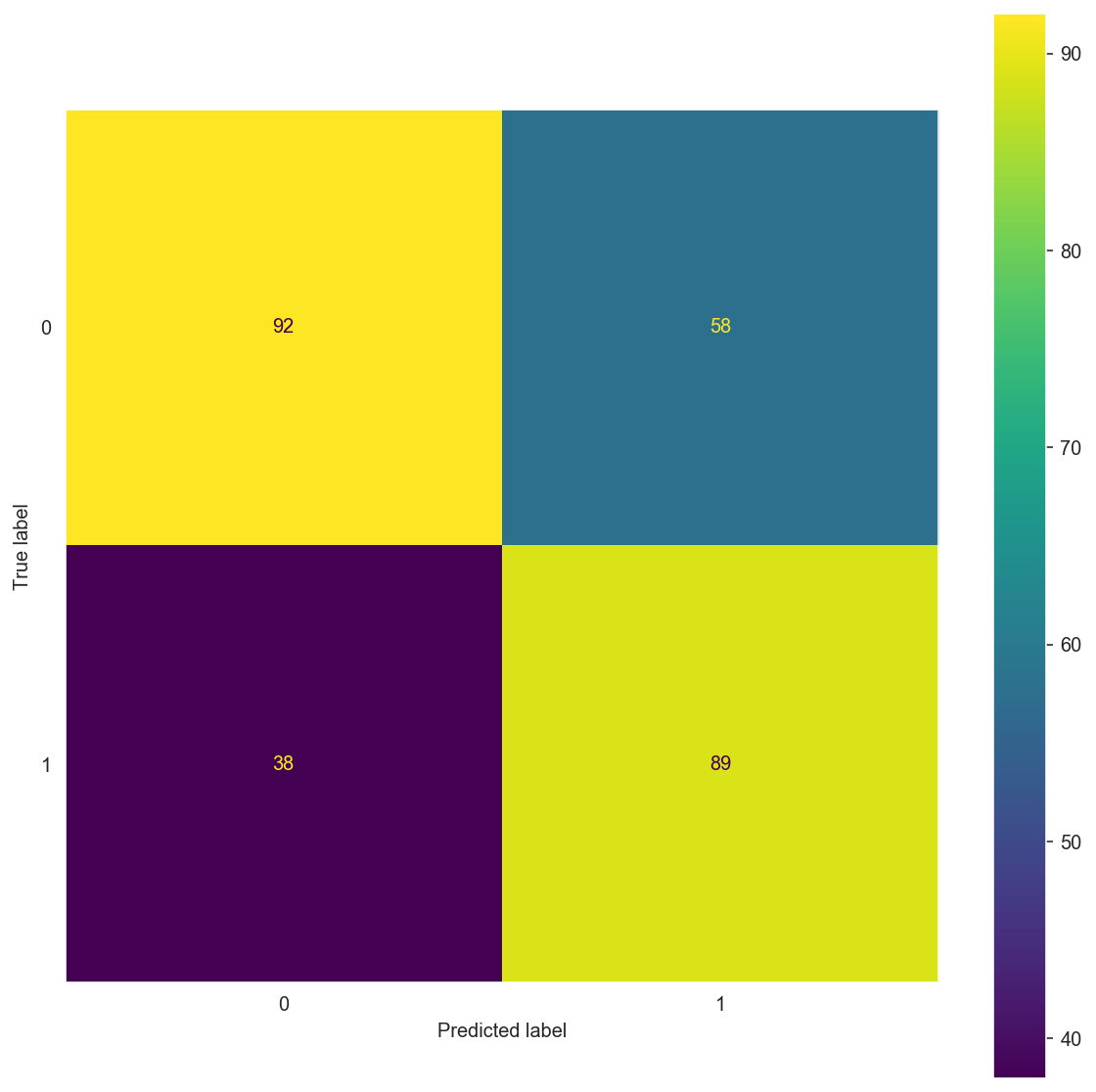
dv = DictVectorizer(sparse=False)
X_dv = dv.fit_transform(df['reduced_stem_count'])
# Sentiment target, convert to 1 for pos, 0 for neg
y_dv = df['Sentiment'].replace('Pos', 1).replace('Neg', 0)
# Break off validation set from training data
X_train_dv, X_test_dv, y_train_dv, y_test_dv = train_test_split(X_dv, y_dv, 
                                        train_size=0.8, test_size=0.2,
                                        random_state=0)
matrix(X_train_dv, y_train_dv, X_test_dv, y_test_dv, alpha=1)

Confusion Matrix:

[[92 58]
 [38 89]]
              precision    recall  f1-score   support

           0       0.71      0.61      0.66       150
           1       0.61      0.70      0.65       127

    accuracy                           0.65       277
   macro avg       0.66      0.66      0.65       277
weighted avg       0.66      0.65      0.65       277

Conclusions

Classification report explained:

• The recall means “how many of this class you find over the whole number of elements of this class”
• The precision will be “how many are correctly classified among that class”
• The f1-score is the harmonic mean between precision & recall
• The support is the number of occurence of the given class in your dataset
• 0 stands for ‘Negative’
• 1 stands for ‘Positive’

Confusion Matrix: \(\begin{bmatrix} TN & FP \\ FN & TP \end{bmatrix}\)

The best confusion matrix has a low:

• False Positive: You predicted positive and it’s false. (Type 1 Error)
• False Negative: You predicted negative and it’s false. (Type 2 Error)

and a high:

• True Positive: You predicted positive and it’s true.
• True Negative: You predicted negative and it’s true.

Model: MultinomialNB()

	precision	recall	f1-score	support
0	0.80	0.75	0.77	150
1	0.73	0.77	0.75	127
accuracy			0.76	277
macro avg	0.76	0.76	0.76	277
weighted avg	0.76	0.76	0.76	277

Confusion Matrix: \(\begin{bmatrix} 113 & 37 \\ 29 & 98 \end{bmatrix}\)

- Hyperparameter Tuning Using KFold() and GridSearch()

Implemented improvements:

• Preprocessed stemmed words with \( N \) occurrences dropped.
• Hyperparameter tuning for \( \alpha=1 \).

	precision	recall	f1-score	support
0	0.82	0.71	0.76	150
1	0.70	0.82	0.76	127
accuracy			0.76	277
macro avg	0.76	0.76	0.76	277
weighted avg	0.77	0.76	0.76	277

Confusion Matrix: \(\begin{bmatrix} 106 & 44 \\ 23 & 104 \end{bmatrix}\)

- Preprocessing Improvement using PorterStemmer()

Implemented improvements:

• Preprocessed stemmed words with \( N<2 \) occurrences dropped.
• Hyperparameter tuning for \( \alpha=10 \).

	precision	recall	f1-score	support
0	0.71	0.65	0.68	150
1	0.62	0.69	0.65	127
accuracy			0.66	277
macro avg	0.66	0.67	0.66	277
weighted avg	0.67	0.66	0.66	277

Confusion Matrix: \(\begin{bmatrix} 97 & 53 \\ 40 & 87 \end{bmatrix}\)

- Using TfidVectorizer()

Implemented improvements:

• Hyperparameter tuning for \( \alpha=0.1 \).
• Use of the TfidVectorizer() instead of the CountVectorizer()

	precision	recall	f1-score	support
0	0.90	0.74	0.81	150
1	0.75	0.91	0.82	127
accuracy			0.82	277
macro avg	0.82	0.82	0.82	277
weighted avg	0.83	0.82	0.82	277

Confusion Matrix: \(\begin{bmatrix} 111 & 39 \\ 12 & 115 \end{bmatrix}\)

Implemented improvements:

• Hyperparameter tuning for \( \alpha=1 \).
• Use of the TfidVectorizer() instead of the CountVectorizer()
• Preprocessed stemmed words with \( N<2 \) occurrences dropped.

	precision	recall	f1-score	support
0	0.74	0.59	0.66	150
1	0.61	0.76	0.68	127
accuracy			0.67	277
macro avg	0.68	0.67	0.67	277
weighted avg	0.68	0.67	0.67	277

Confusion Matrix: \(\begin{bmatrix} 89 & 61 \\ 31 & 96 \end{bmatrix}\)

- Using DictVectorizer()

Implemented improvements:

• Preprocessed stemmed words with \( N<2 \) occurrences dropped.
• Hyperparameter tuning for \( \alpha=10 \).
• Use of the DictVectorizer() instead of the CountVectorizer()

	precision	recall	f1-score	support
0	0.71	0.61	0.66	150
1	0.61	0.70	0.65	127
accuracy			0.65	277
macro avg	0.66	0.66	0.65	277
weighted avg	0.66	0.65	0.65	277

Confusion Matrix: \(\begin{bmatrix} 92 & 58 \\ 38 & 89 \end{bmatrix}\)

For this use case, the TfidVectorizer() with \( \alpha=10 \) allows our model MultinomialNB() to perform better.

- Model: ComplementNB()

ComplementNB() sees a slight decrease in precision, but it shines with imbalanced data sets, and ours is fairly balanced! Should this not be the case with other test train splits, this model should beat MultinomialNB().

Implemented potential improvements:

• Preprocessed stemmed words with \( N<2 \) occurrences dropped.
• Hyperparameter tuning for \( \alpha \).
• Use of the TfidVectorizer() instead of the CountVectorizer()
• Use of the ComplementNB() instead of the MultiNomialNB()

	precision	recall	f1-score	support
0	0.92	0.67	0.77	150
1	0.70	0.93	0.80	127
accuracy			0.79	277
macro avg	0.81	0.80	0.79	277
weighted avg	0.82	0.79	0.78	277

Confusion Matrix: \(\begin{bmatrix} 100 & 50 \\ 9 & 118 \end{bmatrix}\)

Implemented potential improvements:

• Preprocessed stemmed words with \( N<2 \) occurrences dropped.
• Hyperparameter tuning for \( \alpha \).
• Use of the CountVectorizer() instead of the TfidVectorizer()
• Use of the ComplementNB() instead of the MultiNomialNB()

	precision	recall	f1-score	support
0	0.71	0.69	0.70	150
1	0.64	0.67	0.66	127
accuracy			0.68	277
macro avg	0.68	0.68	0.68	277
weighted avg	0.68	0.68	0.68	277

Confusion Matrix: \(\begin{bmatrix} 103 & 47 \\ 42 & 85 \end{bmatrix}\)

Best Results

- Using TfidVectorizer()

Implemented improvements:

• Hyperparameter tuning for \( \alpha=0.1 \).
• Use of the TfidVectorizer() instead of the CountVectorizer()
• No extra preprocessing step to remove word occurrences.

	precision	recall	f1-score	support
0	0.90	0.74	0.81	150
1	0.75	0.91	0.82	127
accuracy			0.82	277
macro avg	0.82	0.82	0.82	277
weighted avg	0.83	0.82	0.82	277

Confusion Matrix: \(\begin{bmatrix} 111 & 39 \\ 12 & 115 \end{bmatrix}\)

References

• [1] J. Nothman, H. Qin and R. Yurchak (2018). “Stop Word Lists in Free Open-source Software Packages”. In Proc. Workshop for NLP Open Source Software.
• [2] Sample pipeline for text feature extraction and evaluation
• [3] Scikit-learn: Machine Learning in Python, Pedregosa et al., JMLR 12, pp. 2825-2830, 2011.