A Single Neuron
Using Keras and Tensorflow we’ll learn how to:
- Create a fully-connected neural network architecture.
- Apply neural nets to two classic ML problems: regression and classification.
- Train neural nets with stochastic gradient descent.
- Improve performance with dropout, batch normalization, and other techniques.
What is Deep Learning?
Some of the most impressive advances in artificial intelligence in recent years have been in the field of deep learning. Natural language translation, image recognition, and game playing are all tasks where deep learning models have neared or even exceeded human-level performance.
So what is deep learning? Deep learning is an approach to machine learning characterized by deep stacks of computations. This depth of computation is what has enabled deep learning models to disentangle the kinds of complex and hierarchical patterns found in the most challenging real-world datasets.
Through their power and scalability neural networks have become the defining model of deep learning. Neural networks are composed of neurons, where each neuron individually performs only a simple computation. The power of a neural network comes instead from the complexity of the connections these neurons can form.
The Linear Unit
So let’s begin with the fundamental component of a neural network: the individual neuron. As a diagram, a neuron (or unit) with one input looks like:
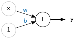
The input is \( x \). Its connection to the neuron has a weight which is \( w \). Whenever a value flows through a connection, you multiply the value by the connection’s weight. For the input \( x \), what reaches the neuron is \( w \times x \). A neural network “learns” by modifying its weights.
The \( b \) is a special kind of weight we call the bias. The bias doesn’t have any input data associated with it; instead, we put a 1 in the diagram so that the value that reaches the neuron is just \( b \) (since \( 1 \times b = b \)). The bias enables the neuron to modify the output independently of its inputs.
The \( y \) is the value the neuron ultimately outputs. To get the output, the neuron sums up all the values it receives through its connections. This neuron’s activation is \( y = w x + b \).
Example - The Linear Unit as a Model
Though individual neurons will usually only function as part of a larger network, it’s often useful to start with a single neuron model as a baseline. Single neuron models are linear models.
Let’s think about how this might work on a dataset like 80 Cereals. Training a model with ‘sugars’ (grams of sugars per serving) as input and ‘calories’ (calories per serving) as output, we might find the bias is \( b=90 \) and the weight is \( w=2.5 \). We could estimate the calorie content of a cereal with 5 grams of sugar per serving like this:
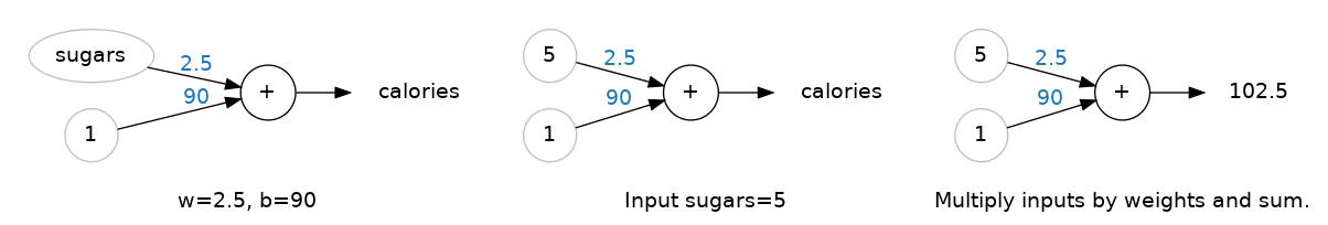
And, checking against our formula, we have calories \( =2.5\times5+90=102.5 \), just like we expect.
Multiple Inputs
The 80 Cereals dataset has many more features than just ‘sugars’. What if we wanted to expand our model to include things like fiber or protein content? That’s easy enough. We can just add more input connections to the neuron, one for each additional feature. To find the output, we would multiply each input to its connection weight and then add them all together.
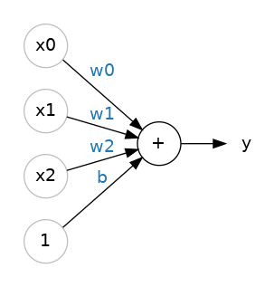
The formula for this neuron would be \( y = w_0 x_0 + w_1 x_1 + w_2 x_2 + b \). A linear unit with two inputs will fit a plane, and a unit with more inputs than that will fit a hyperplane.
Linear Units in Keras
The easiest way to create a model in Keras is through keras.Sequential, which creates a neural network as a stack of layers. We can create models like those above using a dense layer.
We could define a linear model accepting three input features (‘sugars’, ‘fiber’, and ‘protein’) and producing a single output (‘calories’) like so:
from tensorflow import keras
from tensorflow.keras import layers

# Create a network with 1 linear unit
model = keras.Sequential([
    layers.Dense(units=1, input_shape=[3])
])
With the first argument, units, we define how many outputs we want. In this case we are just predicting ‘calories’, so we’ll use units=1.
With the second argument, input_shape, we tell Keras the dimensions of the inputs. Setting input_shape=[3] ensures the model will accept three features as input (‘sugars’, ‘fiber’, and ‘protein’).
Why is input_shape a Python list? The data we’ll use in this course will be tabular data, like in a Pandas dataframe. We’ll have one input for each feature in the dataset. The features are arranged by column, so we’ll always have
input_shape=[num_columns]. The reason Keras uses a list here is to permit use of more complex datasets. Image data, for instance, might need three dimensions:[height, width, channels].