The Sliding Window
In the previous two lessons, we learned about the three operations that carry out feature extraction from an image:
- filter with a convolution layer.
- detect with ReLU activation.
- condense with a maximum pooling layer.
The convolution and pooling operations share a common feature: they are both performed over a sliding window. With convolution, this “window” is given by the dimensions of the kernel, the parameter kernel_size. With pooling, it is the pooling window, given by pool_size.
There are two additional parameters affecting both convolution and pooling layers – these are the strides of the window and whether to use padding at the image edges. The strides parameter says how far the window should move at each step, and the padding parameter describes how we handle the pixels at the edges of the input.
With these two parameters, defining the two layers becomes:
from tensorflow import keras
from tensorflow.keras import layers

model = keras.Sequential([
    layers.Conv2D(filters=64,
                  kernel_size=3,
                  strides=1,
                  padding='same',
                  activation='relu'),
    layers.MaxPool2D(pool_size=2,
                     strides=1,
                     padding='same')
    # More layers follow
])
Stride
The distance the window moves at each step is called the stride. We need to specify the stride in both dimensions of the image: one for moving left to right and one for moving top to bottom. This animation shows strides $=(2, 2)$, a movement of 2 pixels each step
What effect does the stride have? Whenever the stride in either direction is greater than 1, the sliding window will skip over some of the pixels in the input at each step.
Because we want high-quality features to use for classification, convolutional layers will most often have strides$=(1, 1)$. Increasing the stride means that we miss out on potentially valuble information in our summary. Maximum pooling layers, however, will almost always have stride values greater than 1, like $(2, 2)$ or $(3, 3)$, but not larger than the window itself.
Finally, note that when the value of the strides is the same number in both directions, you only need to set that number; for instance, instead of strides$=(2, 2)$, you could use strides$=2$ for the parameter setting.
Padding
When performing the sliding window computation, there is a question as to what to do at the boundaries of the input. Staying entirely inside the input image means the window will never sit squarely over these boundary pixels like it does for every other pixel in the input. Since we aren’t treating all the pixels exactly the same, could there be a problem?
What the convolution does with these boundary values is determined by its padding parameter. In TensorFlow, you have two choices: either padding = ‘same’ or padding = ‘valid’. There are trade-offs with each.
When we set padding = ‘valid’, the convolution window will stay entirely inside the input. The drawback is that the output shrinks (loses pixels), and shrinks more for larger kernels. This will limit the number of layers the network can contain, especially when inputs are small in size.
The alternative is to use padding = ‘same’. The trick here is to pad the input with 0’s around its borders, using just enough 0’s to make the size of the output the same as the size of the input. This can have the effect however of diluting the influence of pixels at the borders. The animation below shows a sliding window with ‘same’ padding.
The VGG model we’ve been looking at uses same padding for all of its convolutional layers. Most modern convnets will use some combination of the two. (Another parameter to tune!)
Example - Exploring Sliding Windows
To better understand the effect of the sliding window parameters, it can help to observe a feature extraction on a low-resolution image so that we can see the individual pixels. Let’s just look at a simple circle.
import tensorflow as tf
import matplotlib.pyplot as plt
plt.rc('figure', autolayout=True)
plt.rc('axes', labelweight='bold', labelsize='large',
titleweight='bold', titlesize=18, titlepad=10)
plt.rc('image', cmap='magma')
image = circle([64, 64], val=1.0, r_shrink=3)
image = tf.reshape(image, [*image.shape, 1])
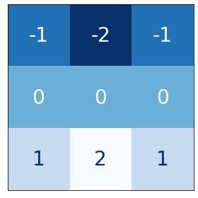
# Bottom sobel
kernel = tf.constant(
[[-1, -2, -1],
[0, 0, 0],
[1, 2, 1]],
)
show_kernel(kernel)
The VGG architecture is fairly simple. It uses convolution with strides of 1 and maximum pooling with $2×2$ windows and strides of 2. We’ve included a function in the visiontools utility script that will show us all the steps.
show_extraction(
    image, kernel,

    # Window parameters
    conv_stride=1,
    pool_size=2,
    pool_stride=2,

    subplot_shape=(1, 4),
    figsize=(14, 6),
)
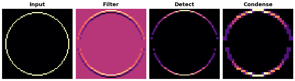
And that works pretty well! The kernel was designed to detect horizontal lines, and we can see that in the resulting feature map the more horizontal parts of the input end up with the greatest activation.
What would happen if we changed the strides of the convolution to 3?
show_extraction(
    image, kernel,

    # Window parameters
    conv_stride=3,
    pool_size=2,
    pool_stride=2,

    subplot_shape=(1, 4),
    figsize=(14, 6),
)
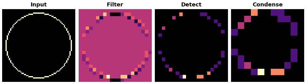
This seems to reduce the quality of the feature extracted. Our input circle is rather “finely detailed,” being only 1 pixel wide. A convolution with strides of 3 is too coarse to produce a good feature map from it.
Sometimes, a model will use a convolution with a larger stride in it’s initial layer. This will usually be coupled with a larger kernel as well. The ResNet50 model, for instance, uses $7×7$ kernels with strides of 2 in its first layer. This seems to accelerate the production of large-scale features without the sacrifice of too much information from the input.
We looked at a characteristic computation common to both convolution and pooling: the sliding window and the parameters affecting its behavior in these layers. This style of windowed computation contributes much of what is characteristic of convolutional networks and is an essential part of their functioning.
Example
In these exercises, you’ll explore the operations a couple of popular convnet architectures use for feature extraction, learn about how convnets can capture large-scale visual features through stacking layers, and finally see how convolution can be used on one-dimensional data, in this case, a time series.
import tensorflow as tf
import matplotlib.pyplot as plt
import learntools.computer_vision.visiontools as visiontools


plt.rc('figure', autolayout=True)
plt.rc('axes', labelweight='bold', labelsize='large',
       titleweight='bold', titlesize=18, titlepad=10)
plt.rc('image', cmap='magma')
Experimenting with Feature Extraction
This exercise is meant to give you an opportunity to explore the sliding window computations and how their parameters affect feature extraction. There aren’t any right or wrong answers – it’s just a chance to experiment!
from learntools.computer_vision.visiontools import edge, blur, bottom_sobel, emboss, sharpen, circle

image_dir = '../input/computer-vision-resources/'
circle_64 = tf.expand_dims(circle([64, 64], val=1.0, r_shrink=4), axis=-1)
kaggle_k = visiontools.read_image(image_dir + str('k.jpg'), channels=1)
car = visiontools.read_image(image_dir + str('car_illus.jpg'), channels=1)
car = tf.image.resize(car, size=[200, 200])
images = [(circle_64, "circle_64"), (kaggle_k, "kaggle_k"), (car, "car")]

plt.figure(figsize=(14, 4))
for i, (img, title) in enumerate(images):
    plt.subplot(1, len(images), i+1)
    plt.imshow(tf.squeeze(img))
    plt.axis('off')
    plt.title(title)
plt.show();

kernels = [(edge, "edge"), (blur, "blur"), (bottom_sobel, "bottom_sobel"),
           (emboss, "emboss"), (sharpen, "sharpen")]
plt.figure(figsize=(14, 4))
for i, (krn, title) in enumerate(kernels):
    plt.subplot(1, len(kernels), i+1)
    visiontools.show_kernel(krn, digits=2, text_size=20)
    plt.title(title)
plt.show()
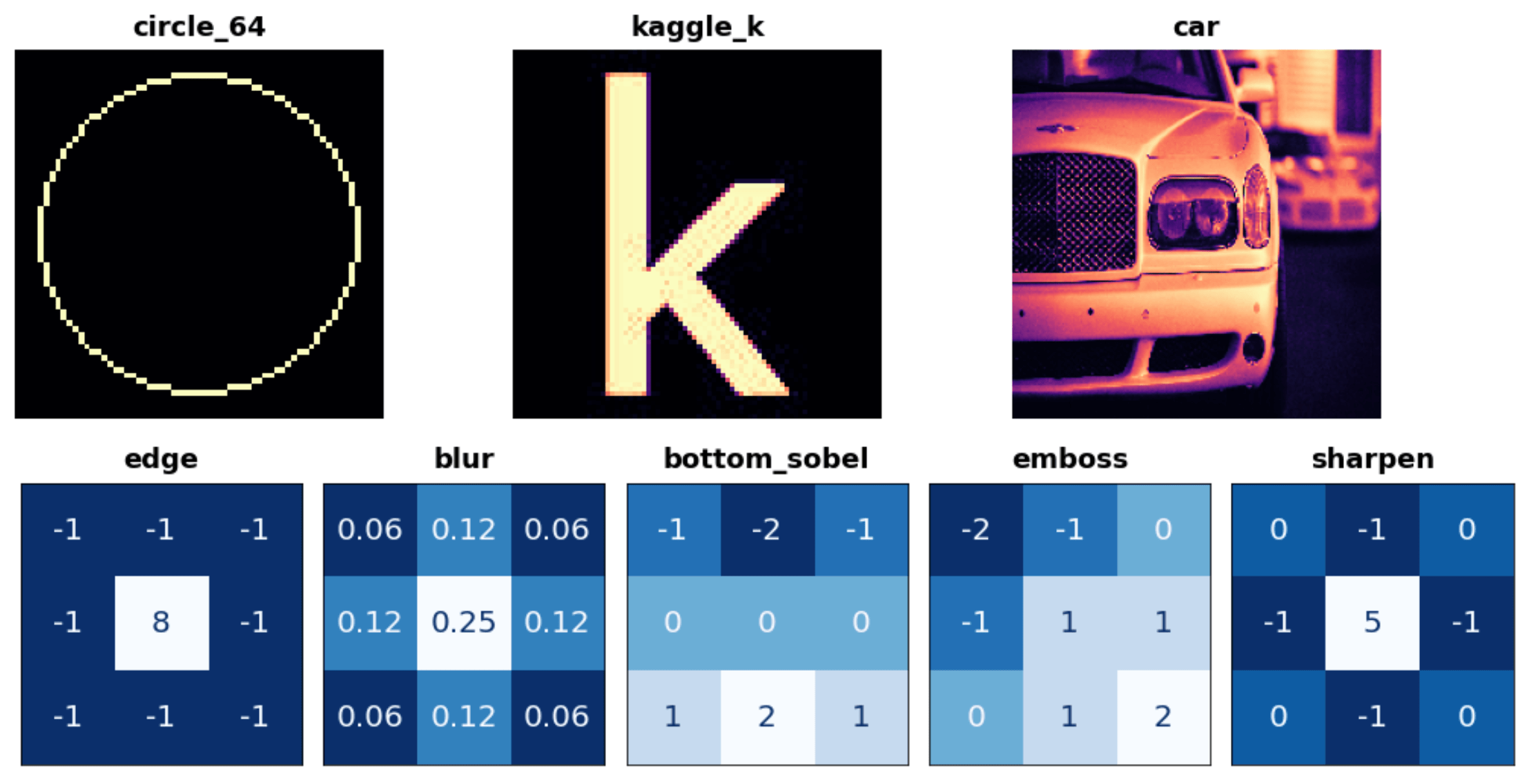
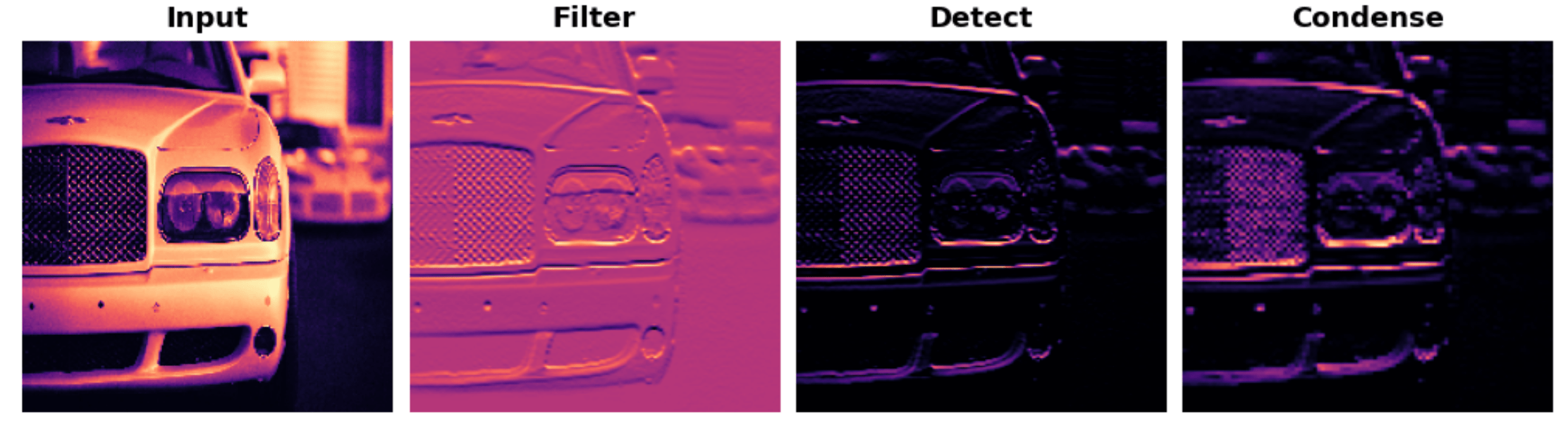
To choose one to experiment with, just enter it’s name in the appropriate place below. Then, set the parameters for the window computation. Try out some different combinations and see what they do!
# YOUR CODE HERE: choose an image
image = car

# YOUR CODE HERE: choose a kernel
kernel = bottom_sobel

visiontools.show_extraction(
    image, kernel,

    # YOUR CODE HERE: set parameters
    conv_stride=1,
    conv_padding='valid',
    pool_size=2,
    pool_stride=2,
    pool_padding='same',

    subplot_shape=(1, 4),
    figsize=(14, 6),
)
The Receptive Field
Trace back all the connections from some neuron and eventually you reach the input image. All of the input pixels a neuron is connected to is that neuron’s receptive field. The receptive field just tells you which parts of the input image a neuron receives information from.
As we’ve seen, if your first layer is a convolution with $3×3$ kernels, then each neuron in that layer gets input from a $3×3$ patch of pixels (except maybe at the border).
What happens if you add another convolutional layer with $3×3$ kernels? Consider this next illustration:
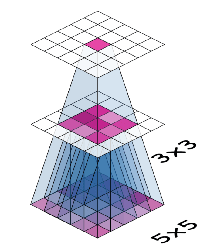
Now trace back the connections from the neuron at top and you can see that it’s connected to a $5×5$ patch of pixels in the input (the bottom layer): each neuron in the $3×3$ patch in the middle layer is connected to a $3×3$ input patch, but they overlap in a $5×5$ patch. So that neuron at top has a $5×5$ receptive field.
Growing the Receptive Field
Now, if you added a third convolutional layer with a $(3, 3)$ kernel, what receptive field would its neurons have?
The third layer would have a $7×7$ receptive field.
So why stack layers like this? Three $(3, 3)$ kernels have $27$ parameters, while one $(7, 7)$ kernel has $49$, though they both create the same receptive field. This stacking-layers trick is one of the ways convnets are able to create large receptive fields without increasing the number of parameters too much.
One-Dimensional Convolution
Convolutional networks turn out to be useful not only (two-dimensional) images, but also on things like time-series (one-dimensional) and video (three-dimensional).
We’ve seen how convolutional networks can learn to extract features from (two-dimensional) images. It turns out that convnets can also learn to extract features from things like time-series (one-dimensional) and video (three-dimensional).
In this (optional) exercise, we’ll see what convolution looks like on a time-series.
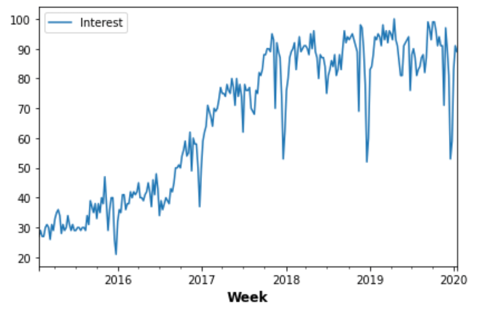
The time series we’ll use is from Google Trends. It measures the popularity of the search term “machine learning” for weeks from January 25, 2015 to January 15, 2020.
import pandas as pd

# Load the time series as a Pandas dataframe
machinelearning = pd.read_csv(
    '../input/computer-vision-resources/machinelearning.csv',
    parse_dates=['Week'],
    index_col='Week',
)

machinelearning.plot();
What about the kernels? Images are two-dimensional and so our kernels were 2D arrays. A time-series is one-dimensional, so what should the kernel be? A 1D array! Here are some kernels sometimes used on time-series data:
detrend = tf.constant([-1, 1], dtype=tf.float32)

average = tf.constant([0.2, 0.2, 0.2, 0.2, 0.2], dtype=tf.float32)

spencer = tf.constant([-3, -6, -5, 3, 21, 46, 67, 74, 67, 46, 32, 3, -5, -6, -3], dtype=tf.float32) / 320
Convolution on a sequence works just like convolution on an image. The difference is just that a sliding window on a sequence only has one direction to travel – left to right – instead of the two directions on an image. And just like before, the features picked out depend on the pattern on numbers in the kernel.
Can you guess what kind of features these kernels extract?
# UNCOMMENT ONE
kernel = detrend
# kernel = average
# kernel = spencer

# Reformat for TensorFlow
ts_data = machinelearning.to_numpy()
ts_data = tf.expand_dims(ts_data, axis=0)
ts_data = tf.cast(ts_data, dtype=tf.float32)
kern = tf.reshape(kernel, shape=(*kernel.shape, 1, 1))

ts_filter = tf.nn.conv1d(
    input=ts_data,
    filters=kern,
    stride=1,
    padding='VALID',
)

# Format as Pandas Series
machinelearning_filtered = pd.Series(tf.squeeze(ts_filter).numpy())

machinelearning_filtered.plot();
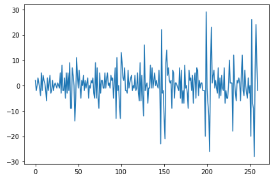
In fact, the detrend kernel filters for changes in the series, while average and spencer are both “smoothers” that filter for low-frequency components in the series.
If you were interested in predicting the future popularity of search terms, you might train a convnet on time-series like this one. It would try to learn what features in those series are most informative for the prediction.
Though convnets are not often the best choice on their own for these kinds of problems, they are often incorporated into other models for their feature extraction capabilities.