Your First Map
In this micro-course, you’ll learn about different methods to wrangle and visualize geospatial data, or data with a geographic location.
Along the way, you’ll offer solutions to several real-world problems like:
- Where should a global non-profit expand its reach in remote areas of the Philippines?
- How do purple martins, a threatened bird species, travel between North and South America? Are the birds travelling to conservation areas?
- Which areas of Japan could potentially benefit from extra earthquake reinforcement?
- Which Starbucks stores in California are strong candidates for the next Starbucks Reserve Roastery location?
- Does New York City have sufficient hospitals to respond to motor vehicle collisions? Which areas of the city have gaps in coverage?
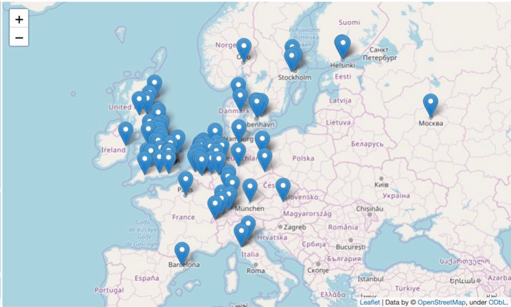
You’ll also visualize crime in the city of Boston, examine health facilities in Ghana, explore top universities in Europe, and track releases of toxic chemicals in the United States.
We’ll also get started with visualizing our first geospatial dataset!
Reading Data
The first step is to read in some geospatial data! To do this, we’ll use the GeoPandas library.
import geopandas as gpd
There are many, many different geospatial file formats, such as shapefile, GeoJSON, KML, and GPKG. We won’t discuss their differences in this micro-course, but it’s important to mention that:
- Shapefile is the most common file type that you’ll encounter.
- All of these file types can be quickly loaded with the gpd.read_file() function.
The next code cell loads a shapefile containing information about forests, wilderness areas, and other lands under the care of the Department of Environmental Conservation in the state of New York.
# Read in the data
full_data = gpd.read_file("../input/geospatial-learn-course-data/DEC_lands/DEC_lands/DEC_lands.shp")

# View the first five rows of the data
full_data.head()
| OBJECTID | CATEGORY | UNIT | FACILITY | CLASS | UMP | DESCRIPTIO | REGION | COUNTY | URL | SOURCE | UPDATE_ | OFFICE | ACRES | LANDS_UID | GREENCERT | SHAPE_AREA | SHAPE_LEN | geometry | |
|---|---|---|---|---|---|---|---|---|---|---|---|---|---|---|---|---|---|---|---|
| 0 | 1 | FOR PRES DET PAR | CFP | HANCOCK FP DETACHED PARCEL | WILD FOREST | None | DELAWARE COUNTY DETACHED PARCEL | 4 | DELAWARE | http://www.dec.ny.gov/ | DELAWARE RPP | 5/12 | STAMFORD | 738.620192 | 103 | N | 2.990365e+06 | 7927.662385 | POLYGON ((486093.245 4635308.586, 486787.235 4… |
| 1 | 2 | FOR PRES DET PAR | CFP | HANCOCK FP DETACHED PARCEL | WILD FOREST | None | DELAWARE COUNTY DETACHED PARCEL | 4 | DELAWARE | http://www.dec.ny.gov/ | DELAWARE RPP | 5/12 | STAMFORD | 282.553140 | 1218 | N | 1.143940e+06 | 4776.375600 | POLYGON ((491931.514 4637416.256, 491305.424 4… |
| 2 | 3 | FOR PRES DET PAR | CFP | HANCOCK FP DETACHED PARCEL | WILD FOREST | None | DELAWARE COUNTY DETACHED PARCEL | 4 | DELAWARE | http://www.dec.ny.gov/ | DELAWARE RPP | 5/12 | STAMFORD | 234.291262 | 1780 | N | 9.485476e+05 | 5783.070364 | POLYGON ((486000.287 4635834.453, 485007.550 4… |
| 3 | 4 | FOR PRES DET PAR | CFP | GREENE COUNTY FP DETACHED PARCEL | WILD FOREST | None | None | 4 | GREENE | http://www.dec.ny.gov/ | GREENE RPP | 5/12 | STAMFORD | 450.106464 | 2060 | N | 1.822293e+06 | 7021.644833 | POLYGON ((541716.775 4675243.268, 541217.579 4… |
| 4 | 6 | FOREST PRESERVE | AFP | SARANAC LAKES WILD FOREST | WILD FOREST | SARANAC LAKES | None | 5 | ESSEX | http://www.dec.ny.gov/lands/22593.html | DECRP, ESSEX RPP | 12/96 | RAY BROOK | 69.702387 | 1517 | N | 2.821959e+05 | 2663.909932 | POLYGON ((583896.043 4909643.187, 583891.200 4… |
As you can see in the “CLASS” column, each of the first five rows corresponds to a different forest.
For the rest of this tutorial, consider a scenario where you’d like to use this data to plan a weekend camping trip. Instead of relying on crowd-sourced reviews online, you decide to create your own map. This way, you can tailor the trip to your specific interests.
Prerequisites
To view the first five rows of the data, we used the head() method. You may recall that this is also what we use to preview a Pandas DataFrame. In fact, every command that you can use with a DataFrame will work with the data!
This is because the data was loaded into a (GeoPandas) GeoDataFrame object that has all of the capabilities of a (Pandas) DataFrame.
type(full_data)
geopandas.geodataframe.GeoDataFrame
For instance, if we don’t plan to use all of the columns, we can select a subset of them.
data = full_data.loc[:, ["CLASS", "COUNTY", "geometry"]].copy()
We use the value_counts() method to see a list of different land types, along with how many times they appear in the dataset.
# How many lands of each type are there?
data.CLASS.value_counts()
WILD FOREST                   965
INTENSIVE USE                 108
PRIMITIVE                      60
WILDERNESS                     52
ADMINISTRATIVE                 17
UNCLASSIFIED                    7
HISTORIC                        5
PRIMITIVE BICYCLE CORRIDOR      4
CANOE AREA                      1
Name: CLASS, dtype: int64
You can also use loc (and iloc) and isin to select subsets of the data.
# Select lands that fall under the "WILD FOREST" or "WILDERNESS" category
wild_lands = data.loc[data.CLASS.isin(['WILD FOREST', 'WILDERNESS'])].copy()
wild_lands.head()
| CLASS | COUNTY | geometry | |
|---|---|---|---|
| 0 | WILD FOREST | DELAWARE | POLYGON ((486093.245 4635308.586, 486787.235 4… |
| 1 | WILD FOREST | DELAWARE | POLYGON ((491931.514 4637416.256, 491305.424 4… |
| 2 | WILD FOREST | DELAWARE | POLYGON ((486000.287 4635834.453, 485007.550 4… |
| 3 | WILD FOREST | GREENE | POLYGON ((541716.775 4675243.268, 541217.579 4… |
| 4 | WILD FOREST | ESSEX | POLYGON ((583896.043 4909643.187, 583891.200 4… |
If you’re not familiar with the commands above, you are encouraged to bookmark this page for reference, so you can look up the commands as needed.
Create your first map!
We can quickly visualize the data with the plot() method.
wild_lands.plot()
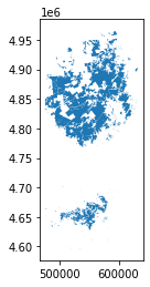
Every GeoDataFrame contains a special “geometry” column. It contains all of the geometric objects that are displayed when we call the plot() method.
# View the first five entries in the "geometry" column
wild_lands.geometry.head()
0    POLYGON ((486093.245 4635308.586, 486787.235 4...
1    POLYGON ((491931.514 4637416.256, 491305.424 4...
2    POLYGON ((486000.287 4635834.453, 485007.550 4...
3    POLYGON ((541716.775 4675243.268, 541217.579 4...
4    POLYGON ((583896.043 4909643.187, 583891.200 4...
Name: geometry, dtype: geometry
While this column can contain a variety of different datatypes, each entry will typically be a Point, LineString, or Polygon.

The “geometry” column in our dataset contains 2983 different Polygon objects, each corresponding to a different shape in the plot above.
In the code cell below, we create three more GeoDataFrames, containing campsite locations (Point), foot trails (LineString), and county boundaries (Polygon).
# Campsites in New York state (Point)
POI_data = gpd.read_file("../input/geospatial-learn-course-data/DEC_pointsinterest/DEC_pointsinterest/Decptsofinterest.shp")
campsites = POI_data.loc[POI_data.ASSET=='PRIMITIVE CAMPSITE'].copy()

# Foot trails in New York state (LineString)
roads_trails = gpd.read_file("../input/geospatial-learn-course-data/DEC_roadstrails/DEC_roadstrails/Decroadstrails.shp")
trails = roads_trails.loc[roads_trails.ASSET=='FOOT TRAIL'].copy()

# County boundaries in New York state (Polygon)
counties = gpd.read_file("../input/geospatial-learn-course-data/NY_county_boundaries/NY_county_boundaries/NY_county_boundaries.shp")
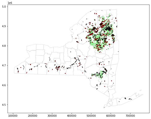
Next, we create a map from all four GeoDataFrames.
The plot() method takes as (optional) input several parameters that can be used to customize the appearance. Most importantly, setting a value for ax ensures that all of the information is plotted on the same map.
# Define a base map with county boundaries
ax = counties.plot(figsize=(10,10), color='none', edgecolor='gainsboro', zorder=3)

# Add wild lands, campsites, and foot trails to the base map
wild_lands.plot(color='lightgreen', ax=ax)
campsites.plot(color='maroon', markersize=2, ax=ax)
trails.plot(color='black', markersize=1, ax=ax)
Example - Kiva.org
Kiva.org is an online crowdfunding platform extending financial services to poor people around the world. Kiva lenders have provided over 1 billion dollars in loans to over 2 million people.
Kiva reaches some of the most remote places in the world through their global network of “Field Partners”. These partners are local organizations working in communities to vet borrowers, provide services, and administer loans.
In this exercise, you’ll investigate Kiva loans in the Philippines. Can you identify regions that might be outside of Kiva’s current network, in order to identify opportunities for recruiting new Field Partners?
import geopandas as gpd

from learntools.core import binder
binder.bind(globals())
from learntools.geospatial.ex1 import *
Use the next cell to load the shapefile located at loans_filepath to create a GeoDataFrame world_loans.
loans_filepath = "../input/geospatial-learn-course-data/kiva_loans/kiva_loans/kiva_loans.shp"

# Your code here: Load the data
world_loans = gpd.read_file(loans_filepath)
| Partner ID | Field Part | sector | Loan Theme | country | amount | geometry | |
|---|---|---|---|---|---|---|---|
| 0 | 9 | KREDIT Microfinance Institution | General Financial Inclusion | Higher Education | Cambodia | 450 | POINT (102.89751 13.66726) |
| 1 | 9 | KREDIT Microfinance Institution | General Financial Inclusion | Vulnerable Populations | Cambodia | 20275 | POINT (102.98962 13.02870) |
| 2 | 9 | KREDIT Microfinance Institution | General Financial Inclusion | Higher Education | Cambodia | 9150 | POINT (102.98962 13.02870) |
| 3 | 9 | KREDIT Microfinance Institution | General Financial Inclusion | Vulnerable Populations | Cambodia | 604950 | POINT (105.31312 12.09829) |
| 4 | 9 | KREDIT Microfinance Institution | General Financial Inclusion | Sanitation | Cambodia | 275 | POINT (105.31312 12.09829) |
# This dataset is provided in GeoPandas
world_filepath = gpd.datasets.get_path('naturalearth_lowres')
world = gpd.read_file(world_filepath)
world.head()
| pop_est | continent | name | iso_a3 | gdp_md_est | geometry | |
|---|---|---|---|---|---|---|
| 0 | 920938 | Oceania | Fiji | FJI | 8374.0 | MULTIPOLYGON (((180.00000 -16.06713, 180.00000… |
| 1 | 53950935 | Africa | Tanzania | TZA | 150600.0 | POLYGON ((33.90371 -0.95000, 34.07262 -1.05982… |
| 2 | 603253 | Africa | W. Sahara | ESH | 906.5 | POLYGON ((-8.66559 27.65643, -8.66512 27.58948… |
| 3 | 35623680 | North America | Canada | CAN | 1674000.0 | MULTIPOLYGON (((-122.84000 49.00000, -122.9742… |
| 4 | 326625791 | North America | United States of America | USA | 18560000.0 | MULTIPOLYGON (((-122.84000 49.00000, -120.0000… |
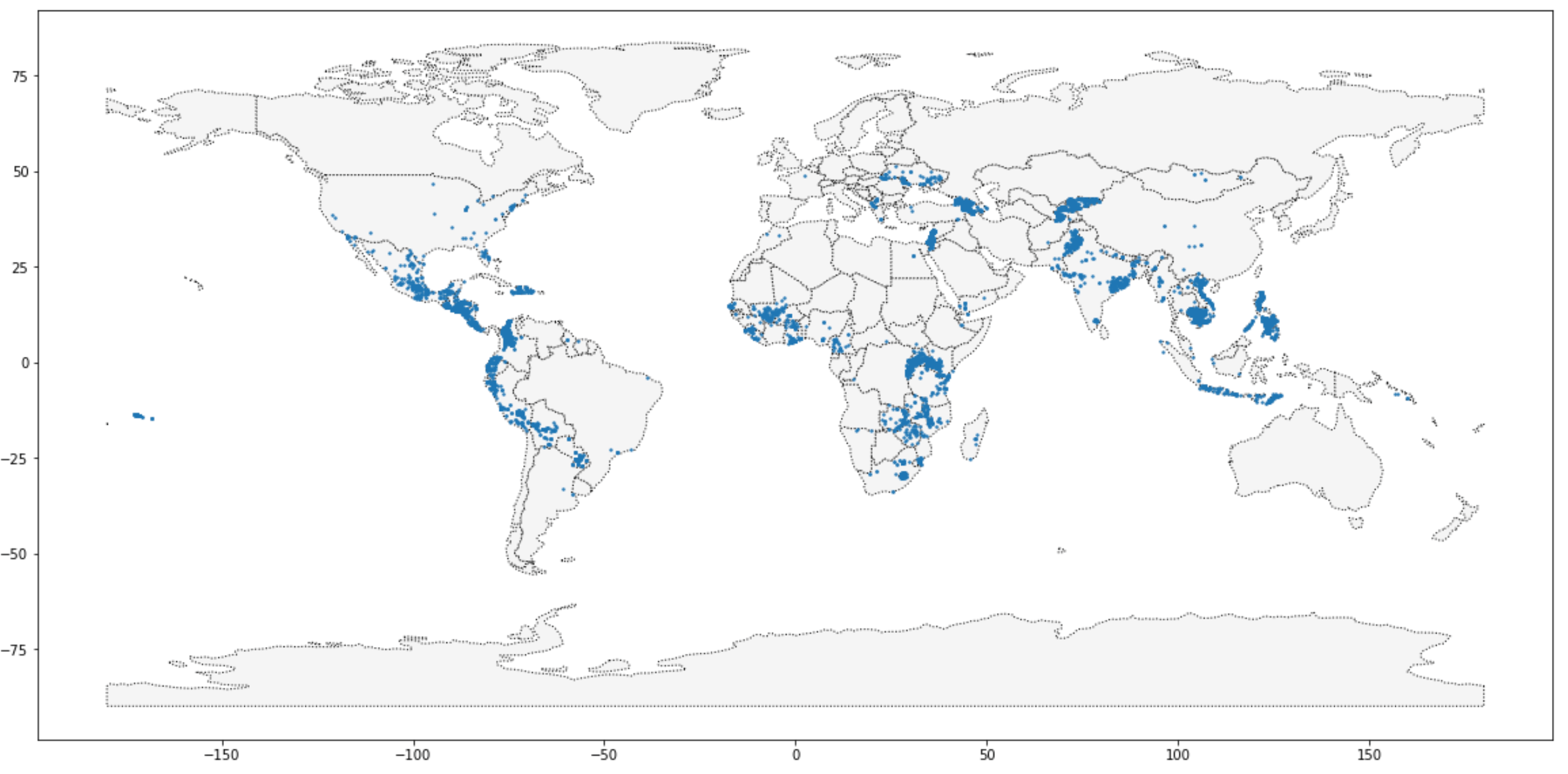
Use the world and world_loans GeoDataFrames to visualize Kiva loan locations across the world.
# Your code here
ax = world.plot(figsize=(20,20), color='whitesmoke', linestyle=':', edgecolor='black')
world_loans.plot(ax=ax, markersize=2)
PHL_loans = world_loans.loc[world_loans.country=="Philippines"].copy()
# Load a KML file containing island boundaries
gpd.io.file.fiona.drvsupport.supported_drivers['KML'] = 'rw'
PHL = gpd.read_file("../input/geospatial-learn-course-data/Philippines_AL258.kml", driver='KML')
PHL.head()
| Name | Description | geometry | |
|---|---|---|---|
| 0 | Autonomous Region in Muslim Mindanao | MULTIPOLYGON (((119.46690 4.58718, 119.46653 4… | |
| 1 | Bicol Region | MULTIPOLYGON (((124.04577 11.57862, 124.04594 … | |
| 2 | Cagayan Valley | MULTIPOLYGON (((122.51581 17.04436, 122.51568 … | |
| 3 | Calabarzon | MULTIPOLYGON (((120.49202 14.05403, 120.49201 … | |
| 4 | Caraga | MULTIPOLYGON (((126.45401 8.24400, 126.45407 8… |
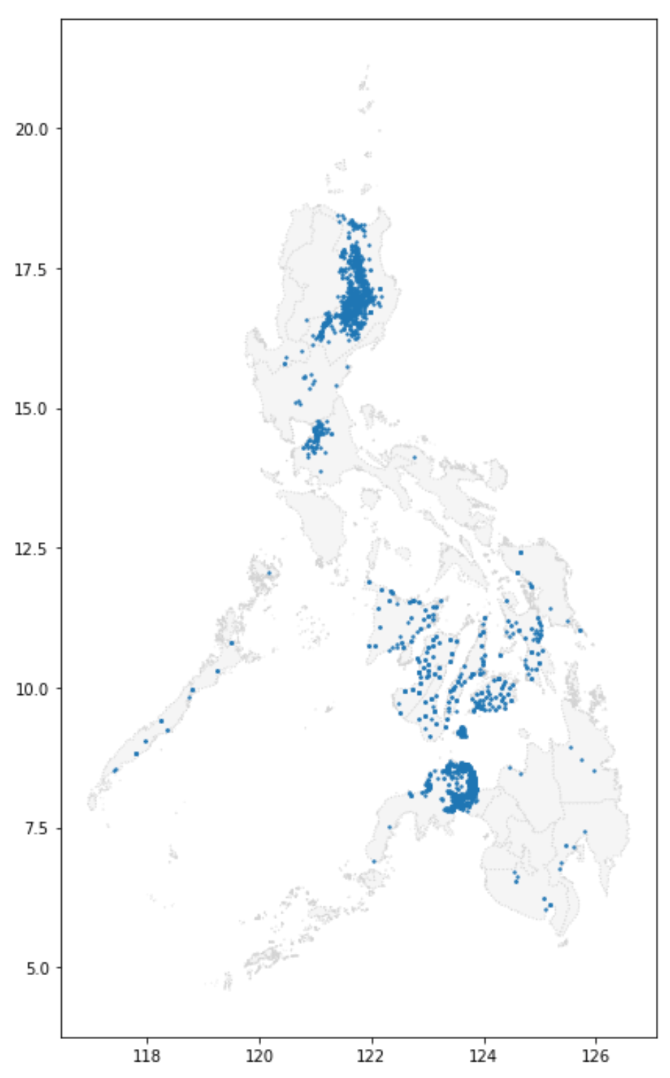
Can you identify any islands where it might be useful to recruit new Field Partners? Do any islands currently look outside of Kiva’s reach?
There are a number of potential islands, but Mindoro (in the central part of the Philippines) stands out as a relatively large island without any loans in the current dataset. This island is potentially a good location for recruiting new Field Partners!